• Skip to main content
  • Skip to primary sidebar
  • Skip to secondary sidebar
  • Skip to footer

Computer Notes

Library
    • Computer Fundamental
    • Computer Memory
    • DBMS Tutorial
    • Operating System
    • Computer Networking
    • C Programming
    • C++ Programming
    • Java Programming
    • C# Programming
    • SQL Tutorial
    • Management Tutorial
    • Computer Graphics
    • Compiler Design
    • Style Sheet
    • JavaScript Tutorial
    • Html Tutorial
    • Wordpress Tutorial
    • Python Tutorial
    • PHP Tutorial
    • JSP Tutorial
    • AngularJS Tutorial
    • Data Structures
    • E Commerce Tutorial
    • Visual Basic
    • Structs2 Tutorial
    • Digital Electronics
    • Internet Terms
    • Servlet Tutorial
    • Software Engineering
    • Interviews Questions
    • Basic Terms
    • Troubleshooting
Menu

Header Right

Home » Graphics » Simple Line Drawing Method

What is FatBits?

By Dinesh Thakur

On the Macintosh, some programs let you edit bitmapped graphics as FatBits. In FatBits mode, the individual dots, or pixels, making up the image are blown up so you can work with them easily, one at a time. If you see stray dots in an image you’ve scanned, or if a line in a picture is just slightly too thick or too skinny, it’s almost impossible to make precise changes working at normal size.


Traditionally, you can get into FatBits mode by selecting the pencil tool, holding down the Command key, and clicking on the image at the spot you want to see enlarged. You might also have a magnifying glass tool, or a menu command for FatBits or a command to Enlarge. Sometimes to get out of FatBits you can hold down the Option key and click.
What is Duotone?

By Dinesh Thakur

A typical black-and-white photograph uses only one color. In a duotone, though, the black-and-white photograph (or other artwork) is reproduced using two colors. Perhaps it’s black and brown, or black and grey, or dark grey and a rusty color. Halftone images are generated for the photograph, one slightly underexposed and one slightly overexposed, and the two are printed one on top of the other. The result can be an incredibly rich, powerful image-much richer and more interesting than the image with one color. The artist/designer has control over the values and percentages of the two different colors. It is also possible to make “tritones” using three different colors, and “quadtones,” using four different colors.


A duotone (or tritone or quadtone) does not refer to the use of spot color for the second color; that is, if you take a photograph and color the lady’s dress pink, that’s not a duotone, even though there are two colors in the image.

What is Dot Gain?

By Dinesh Thakur

Whenever a photograph, painting or drawing containing many colors or gray tones is printed, the colors and tones must be simulated with tiny dots. Dot gain refers to an increase in the size of these dots when they are actually printed on the paper by the printing press. The dots can increase in size rather dramatically once the ink hits the paper, depending on the characteristics of the press, the absorbency of the paper, and the nature of the ink that is used.


The effect of dot gain on the final printed piece can be an increase in color intensity, because more ink is put on the paper (by the press) than was called for when the image was output, making the colors look darker than intended. Because the dots have gained in size, the final printed image can look not only darker, but muddy, low in contrast, and blurry.

The best of the color separation utilities offer a way to compensate for dot gain by adjusting the color curves when the film is imaged, but sometimes the artist has to compensate for dot gain manually within the software application used to create the image. It helps if the artist, the commercial press, and the service bureau work together closely so they can adjust for the quirks of each others’ equipment and compensate for the dot gain effectively

What is Antialiasing?

By Dinesh Thakur

When text or a graphic image is displayed on amonitor,or screen, the smoothness of the edges is limited by the resolution of the screen, which means the edges tend to be a little jagged. This jaggedness is also called aliasing.

There are a variety of techniques used to reduce the jaggies, or the aliasing of text and graphic images, to fool our eyes into thinking the edge is smoother. For instance, in animage editingprogram you can blur the edges, or shade along the lines to make the dark-to-light transition less distinct.Anti-aliasing, then, means to use one of these techniques to smooth out the rough edges (the aliasing).

Antialiasing: A technique employed in computer GRAPHICS to smooth the jagged appearance of text and lines by applying varying shades of colour. Consider a black diagonal line drawn on a white screen background: on a low RESOLUTION display it will appear stepped like a staircase because the positions of screen pixels will not coincide exactly with the desired path of the line. On a screen that can display shades of grey, anti aliasing involves coloring each pixel black if it lies wholly within the line, white if it lies wholly outside the line, but otherwise a shade of grey proportional to the degree with which it overlaps the line.

The same principle works with any foreground and background colour combination, by exploiting a property of the human eye that expects the edges of objects to display some tonal gradation due to light and shadow. Antialiased text is a feature of most sophisticated text processing and design software.

Scan converting a point

By Dinesh Thakur

A mathematical point (x, y) where x and y are real numbers within an image area, needs to be scan converted to a pixel at location (x’, y’). This may be done by making x’ to be the integer part of x, and y’ to be the integer part of y. In other words, x’ = floor(x) and y’ = floor(y),

 where function floor returns the largest integer that is less than or equal to the arguments. Doing so in essence places the origin of a continuous coordinate system for (x, y) at the lower left corner of the pixel grid in the image space. All the points that satisfy x’? x ? x’ + 1 and y’? y ? y’ + 1 are mapped to pixel (x’, y’). Let us take for example a point P1(1.7, 0.8).


It will be represented by pixel (1, 0). Points P2 (2.2, 1.3) and P3(2.8, 1.9) are both represented by pixel (2, 1). Let us take another approach to align the integer values in the coordinate system for (x, y) with the pixel coordinates. Here we can convert (x, y) by making x’ = floor(x + 0.5) and y’ = floor(y + 0.5). This approach places the origin of the coordinate system for (x, y) at the center of pixel(0,0).


All points that satisfy x’- 0.5 ? x ? x’+0.5 and y’- 0.5 ? y ? y’+0.5 are mapped to pixel (x’, y’). This means that points P1 and P2 are now both represented by pixel (2, 1), whereas point P3 is represented by pixel (3, 2).


Scan Converting a Line

By Dinesh Thakur

You know that a line in computer graphics typically refers to a line segment, which is a portion of a straight line that extends indefinitely in opposite directions. You can define a line by its two end points and by the line equation y = mx + c, where m is called the slope and c the y intercept of the line. Let the two end points of a line be P1(x1, y1) and P2(x2, y2). The line equation describes the coordinates of all the points that lie between the two endpoints.

 A simple approach to scan convert a line is to first scan convert P1 and P2 to pixel coordinates (x1’, y1’) and (x2’, y2’) respectively. Then let us set m = (y2’- y1’)/(x2’- x1’) and b = y1’-mx1’. Find |m| and if |m| ? 1, then for every integer value of x between and excluding x1’ and x2’, calculate the corresponding value of y using the equation and scan convert (x, y). If |m| >1, then for every integer value of y between and excluding y1’ and y2’, calculate the corresponding value of x using the equation and scan convert (x, y).


Design criteria of straight lines


From geometry we know that a line, or line segment, can be uniquely specified by two points. From algebra we also know that a line can be specified by a slope, usually given the name m and a y-axis intercept called b. Generally in computer graphics, a line will be specified by two endpoints. But the slope and y-intercept are often calculated as intermediate results for use by most line-drawing algorithms.


The goal of any line drawing algorithm is to construct the best possible approximation of an ideal line given the inherent limitations of a raster display. Before discussing specific line drawing algorithms, it is useful to consider general requirements for such algorithms. Let us see what are the desirable characteristics needed for these lines.


The primary design criteria are as follows


  • Straight lines appear as straight lines
  • Straight lines start and end accurately
  • Displayed lines should have constant brightness along their length, independent of the line length and orientation.
  • Lines should be drawn rapidly

Write Short Note on Digital Differential Analyzer (DDA)

By Dinesh Thakur

DDA algorithm is an incremental scan conversion method. Here we perform calculations at each step using the results from the preceding step. The characteristic of the DDA algorithm is to take unit steps along one coordinate and compute the corresponding values along the other coordinate. The unit steps are always along the coordinate of greatest change, e.g. if dx = 10 and dy = 5, then we would take unit steps along x and compute the steps along y.

 Suppose at step i we have calculated (xi, yi) to be a point on the line. Since the next point (x i+1,y i+1) should satisfy ?y/? x =m where ?y= y i+1–yi and ? x= x i+1–xi , we have y i+1= yi + m? x or x i+1=xi+ ? y/m

 These formulas are used in DDA algorithm as follows. When |m| ? 1, we start with x = x1’? (assuming that x1’ <x2’) and y = y1’, and set ? x =1( i.e., unit increment in the x direction). The y coordinate of each successive point on the line is calculated using y i+1= yi + m.

When |m| >1, we start with x= x1’ and y= y1’ (assuming that y1’ < y2’), set ? y =1 ( i.e., unit increment in the y direction). The x coordinate of each successive point on the line is calculated using x i+1=xi+ 1/m. This process continues until x reaches x2’(for m| ? 1 case )or y reaches y2’ (for m| > 1 case ) and all points are scan converted to pixel points.

The explanation is as follows: In DDA algorithm we have to find the new point xi+1 and yi+1 from the existing points xi and yi. As a first step here we identify the major axis and the minor axis of the line to be drawn. Once the major axis is found we sample the major axis at unit intervals and find the value in the other axis by using the slope equation of the line.

For example if the end points of the line is given as (x1,y1)= (2,2) and (x2, y2)= (9,5). Here we will calculate y2-y1 and x2-x1 to find which one is greater. Here y2-y1 =3 and x2-x1 =7; therefore here the major axis is the x axis. So here we need to sample the x axis at unit intervals i.e.? x = 1 and we will find out the y values for each ? x in the x axis using the slope equation.

 In DDA we need to consider two cases; one is slope of the line less than or equal to one (|m| ? 1)and slope of the line greater than one (m| > 1). When |m| ? 1 means y2-y1 = x2-x1 or y2-y1 <x2-x1.In both these cases we assume x to be the major axis. Therefore we sample x axis at unit intervals and find the y values corresponding to each x value.

We have the slope equation as

? y = m ? x

           y2-y1 = m (x2-x1)

In general terms we can say that y i+1 – yi = m(x i+1 – xi ). But here ? x = 1; therefore the equation reduces to y i+1= yi + m = yi + dy/dx.

When m| > 1 means y2-y1> x2-x1 and therefore we assume y to be the major axis. Here

we sample y axis at unit intervals and find the x values corresponding to each y value. We have the slope equation as

? y = m ? x

y2-y1 = m (x2-x1)

In general terms we can say that y i+1 – yi = m(x i+1 – xi ). But here ? y = 1; therefore the equation reduces to 1 = m(x i+1 – xi). Therefore

x i+1=xi+ 1/m

x i+1=xi+ dx/dy

DDA Algorithm is given below:

procedure DDA( x1, y1, x2, y2: integer);

var

            dx, dy, steps: integer;

            x_inc, y_inc, x, y: real;

begin

            dx := x2 – x1; dy := y2 – y1;

            if abs(dx) > abs(dy) then

            steps := abs(dx); {steps is larger of dx, dy}

else

            steps := abs(dy);

            x_inc := dx/steps; y_inc := dy/steps;

            {either x_inc or y_inc = 1.0, the other is the slope}

            x:=x1; y:=y1;

            set_pixel(round(x), round(y));

            for i := 1 to steps do

begin

             x := x + x_inc;

             y := y + y_inc;

              set_pixel(round(x), round(y));

end;

end; {DDA}

The DDA algorithm is faster than the direct use of the line equation since it calculates points on the line without any floating point multiplication.

Advantages of DDA Algorithm

1. It is the simplest algorithm and it does not require special skills for implementation.
2. It is a faster method for calculating pixel positions than the direct use of equation y = mx + b. It eliminates the multiplication in the equation by making use of raster characteristics, so that appropriate increments are applied in the x or v direction to find the pixel positions along the line path.

Disadvantages of DDAAlgorithm

1. Floating point arithmetic in DDA algorithm is still time-consuming.
2. The algorithm is orientation dependent. Hence end point accuracy is poor.

Let us see few examples to illustrate this algorithm.


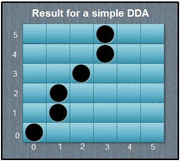
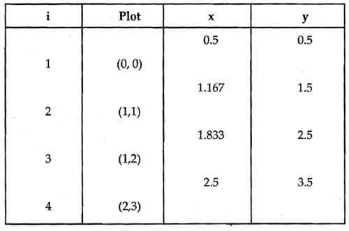
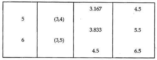
Consider the line from (0,0) to (4,6). Use the simple DDA algorithm to rasterize this line.


Sol. Evaluating steps 1 to 5 in the DDA algorithm we have


Xl = 0                          Y1 = 0

X2 = 4                          Y2 = 6

Length = |Y2-Y1l = 6

                             ∆X = |X2– Xl | / Length

                                 =       4

                                           6

                             ∆Y = |Y2– Yl | / Length

                                   = 6/6=1

Initial value for

                               X = 0 + 0.5 * Sign (4) = 0.5

                                                                 6

                               Y = 0 + 0.5 * Sign (1) = 0.5


Tabulating the results of each iteration in the step 6 we get,

                         DDA Algorithm

                         DDA-Algo

                                             Result for a simple DDA


The results are plotted as shown in the Fig. It shows that the rasterized line lies to both sides of the actual line, i.e. the algorithm is orientation dependent.


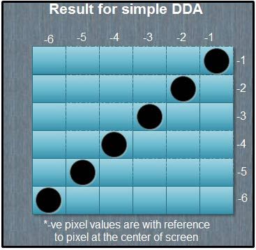
Example 2 Consider the line from (0, 0) to (-6, -6). Use the simple DDA algorithm line.


Sol. Evaluating steps 1 to 5 in the DDA algorithm we have


Xl = 0                          Y1 = 0

X2 = – 6                       Y2 = – 6                  

Length = l X2-X1l |Y2-Y1l = 6

                           ∆X = ∆Y = -1

Initial values for

                                       X = 0 + 0.5 * Sign (-1) =-0.5

                                       Y = 0 + 0.5 * Sign (-1) =-0.5

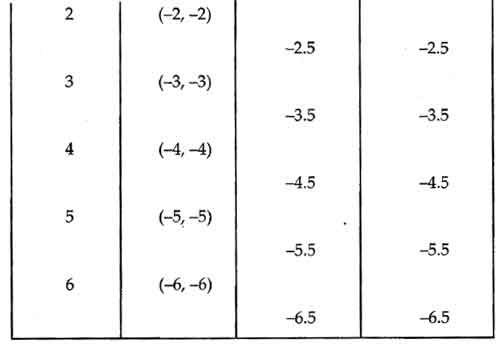
Tabulating the results of each iteration in the step 6 we get,

                             DDA Algorithm Line

                             DDA Algorithm Lines

                                                Result for simple DDA

The results are plotted as shown in the Fig. It shows that the rasterized line lies on the actual line and it is 45° line.


Bresenham’s Line Drawing Algorithm.

By Dinesh Thakur

You know that DDA algorithm is an incremental scan conversion method which performs calculations at each step using the results from the preceding step. Here we are going to discover an accurate and efficient raster line generating algorithm, the Bresenham’s line-drawing algorithm.

This algorithm was developed by Jack E. Bresenham in 1962 at IBM. As stated above, in this lecture, I will explain how to draw lines using the Bresenham’s line-drawingalgorithm. And then show you the complete line drawing function. Before we begin on this topic, a revision of the concepts developed earlier like scan conversion methods and rasterization may be helpful. Once we finish this aspect, we will proceed towards exposition of items listed in the synopsis.

In particular, we will emphasize the following

(a) The working of Bresenham’s algorithm.

(b) Implementation of the Bresenham’s algorithm.

The working of Bresenham’s algorithm The following is an explanation of how the Bresenham’s line-drawing algorithm works, rather than exact implementation.

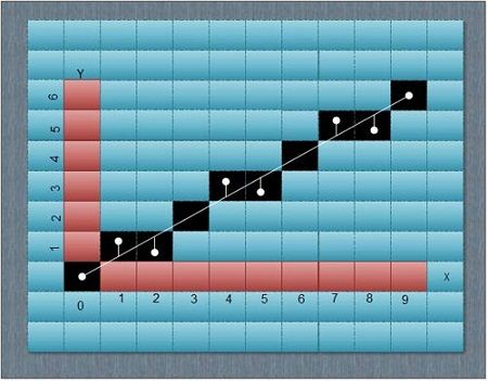
                   Bresenhams line drawing Algorithm

Let’s take a look at this image. One thing to note here is that it is impossible to draw the true line that we want because of the pixel spacing. Putting it in other words, there’s no enough precision for drawing true lines on a PC monitor especially when dealing with low resolutions. The Bresenham’s line-drawing algorithm is based on drawing an approximation of the true line. 

The true line is indicated in bright color, and its approximation is indicated in black pixels. In this example the starting point of the line is located exactly at 0, 0 and the ending point of the line is located exactly at 9, 6. Now let discuss the way in which this algorithm works. First it decides which axis is the major axis and which is the minor axis.

The major axis is longer than the minor axis. On this picture illustrated above the major axis is the X axis. Each iteration progresses the current value of the major axis (starting from the original position), by exactly one pixel. Then it decides which pixel on the minor axis is appropriate for the current pixel of the major axis. Now how can you approximate the right pixel on the minor axis that matches the pixel on the major axis?

That’s what Bresenham’s line-drawing algorithm is all about. And it does so by checking which pixel’s center is closer to the true line. Now you take a closer look at the picture. The center of each pixel is marked with a dot. The algorithm takes the coordinates of that dot and compares it to the true line. If the span from the center of the pixel to the true line is less or equal to 0.5, the pixel is drawn at that location. That span is more generally known as the error term.

You might think of using floating variables but you can see that the whole algorithm is done in straight integer math with no multiplication or division in the main loops(no fixed point math either). Now how is it possible? Basically, during each iteration through the main drawing loop the error term is tossed around to identify the right pixel as close as possible to the true line. Let’s consider these two deltas between the length and height of the line: dx = x1 – x0; dy = y1 – y0; 

This is a matter of precision and since we’re working with integers you will need to scale the deltas by 2 generating two new values: dx2 = dx*2; dy2 = dy*2; These are the values that will be used to change the error term. Why do you scale the deltas? That’s because the error term must be first initialized to 0.5 and that cannot be done using an integer. Finally the scaled values must be subtracted by either dx or dy (the original, non-scaled delta values) depending on what the major axis is (either x or y).

The implementation of Bresenham’s algorithm

The function given below handles all lines and implements the complete Bresenham’s algorithm.

function line(x0, x1, y0, y1)

boolean steep := abs(y1 – y0) > abs(x1 – x0)

if steep then

swap(x0, y0)

swap(x1, y1)

if x0 > x1 then

swap(x0, x1)

swap(y0, y1)

int deltax := x1 – x0

int deltay := abs(y1 – y0)

real error := 0

real deltaerr := deltay / deltax

int y := y0

if y0 < y1 then ystep := 1 else ystep := -1

for x from x0 to x1

if steep then plot(y,x) else plot(x,y)

error := error + deltaerr

if error ? 0.5

y := y + ystep

error := error – 1.0

Note:-To draw lines with a steeper slope, we take advantage of the fact that a steep line can be reflected across the line y=x to obtain a line with a small slope. The effect is to switch the x and y variables throughout, including switching the parameters to plot.


Primary Sidebar

Computer Graphics Tutorials

Computer Graphics

  • CG - Home
  • CG - Introduction
  • CG - Applications
  • CG - Applications
  • CG - Raster Vs Random Scan Display
  • CG - Frame Buffer
  • CG - DVST
  • CG - CRT Display
  • CG - DDA
  • CG - Transformation
  • CG - Cathode Ray Tube
  • CG - Bresenham’s Line Algorithm
  • CG - Pixel
  • CG - Data Compression
  • CG - Clipping
  • CG - Shadow Mask CRT
  • CG - Line Drawing Algorithm
  • CG - Text Clipping
  • CG - Refresh Rates
  • CG - CRT/Monitor
  • CG - Interactive Graphics Display
  • CG - Raster Vs Random Scan System
  • CG - Liquid Crystal Display
  • CG - Scan Converting a Line
  • CG - Monitors Types
  • CG - Display Types
  • CG - Sutherland-Hodgeman Clipping
  • CG - Bitmap
  • CG - Antialiasing
  • CG - Refresh Rates
  • CG - Shadow Mask Vs Beam Penetration
  • CG - Scan Converting a Point
  • CG - Image Resolution
  • CG - Double Buffering
  • CG - Raster Vs Random Scan
  • CG - Aspect Ratio
  • CG - Ambient Light
  • CG - Image Processing
  • CG - Interactive Graphics Displayed
  • CG - Shadow Mask CRT
  • CG - Dithering
  • CG - GUI
  • CG - CLUT
  • CG - Graphics
  • CG - Resolutions Types
  • CG - Transformations Types
  • CG - Half-toning Effect
  • CG - VGA
  • CG - Aliasing
  • CG - CGA

Other Links

  • Computer Graphics - PDF Version

Footer

Basic Course

  • Computer Fundamental
  • Computer Networking
  • Operating System
  • Database System
  • Computer Graphics
  • Management System
  • Software Engineering
  • Digital Electronics
  • Electronic Commerce
  • Compiler Design
  • Troubleshooting

Programming

  • Java Programming
  • Structured Query (SQL)
  • C Programming
  • C++ Programming
  • Visual Basic
  • Data Structures
  • Struts 2
  • Java Servlet
  • C# Programming
  • Basic Terms
  • Interviews

World Wide Web

  • Internet
  • Java Script
  • HTML Language
  • Cascading Style Sheet
  • Java Server Pages
  • Wordpress
  • PHP
  • Python Tutorial
  • AngularJS
  • Troubleshooting

 About Us |  Contact Us |  FAQ

Dinesh Thakur is a Technology Columinist and founder of Computer Notes.

Copyright © 2025. All Rights Reserved.

APPLY FOR ONLINE JOB IN BIGGEST CRYPTO COMPANIES
APPLY NOW