• Skip to main content
  • Skip to primary sidebar
  • Skip to secondary sidebar
  • Skip to footer

Computer Notes

Library
    • Computer Fundamental
    • Computer Memory
    • DBMS Tutorial
    • Operating System
    • Computer Networking
    • C Programming
    • C++ Programming
    • Java Programming
    • C# Programming
    • SQL Tutorial
    • Management Tutorial
    • Computer Graphics
    • Compiler Design
    • Style Sheet
    • JavaScript Tutorial
    • Html Tutorial
    • Wordpress Tutorial
    • Python Tutorial
    • PHP Tutorial
    • JSP Tutorial
    • AngularJS Tutorial
    • Data Structures
    • E Commerce Tutorial
    • Visual Basic
    • Structs2 Tutorial
    • Digital Electronics
    • Internet Terms
    • Servlet Tutorial
    • Software Engineering
    • Interviews Questions
    • Basic Terms
    • Troubleshooting
Menu

Header Right

Home » DS » Data Structures

Graphs

Trees

Queues

Searching and Sorting

Linked Lists

Basic of Data Structure

Data Structures

Using free() Function in C

By Dinesh Thakur

The function free() is used to de-allocate the memory allocated by the functions malloc ( ), calloc ( ), etc, and return it to heap so that it can be used for other purposes. The argument of the function free ( ) is the pointer to the memory which is to be freed. The prototype of the function is as below.

void free(void *ptr);

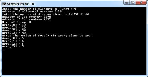
When free () is used for freeing memory allocated by malloc () or realloc (),the whole allocated memory block is released. For the memory allocated by function calloc () also all the segments of memory allocated by calloc () are de-allocated by free (). This is illustrated by Program. The following program demonstrates the use of function calloc () and the action of function free () on the memories allocated by calloc () .

Illustrates that function free () frees all blocks of memory allocated by calloc () function

#include <stdio.h> 
#include<stdlib.h>
main()
{
   int i,j,k, n ;
   int* Array;
   clrscr();
   printf("Enter the number of elements of Array : ");
   scanf("%d", &n );
   Array= (int*) calloc(n, sizeof(int));
   if( Array== (int*)NULL)
     {
         printf("Error. Out of memory.\n");
         exit (0);
      }
       printf("Address of allocated memory= %u\n" , Array);
       printf("Enter the values of %d array elements:", n);
        for (j =0; j<n; j++)
             scanf("%d",&Array[j]);
             printf("Address of Ist member= %u\n", Array);
             printf("Address of 2nd member= %u\n", Array+1);
             printf("Size of Array= %u\n", n* sizeof(int) );
     for ( i = 0 ; i<n; i++)
       printf("Array[%d] = %d\n", i, *(Array+i));
       free(Array);
       printf("After the action of free() the array elements are:\n");
       for (k =0;k<n; k++)
          printf("Array[%d] = %d\n", k, *(Array+i));
          return 0;
}

Memory Allocation Function Calloc()

By Dinesh Thakur

The function is used to allocate contiguous blocks of memory of same size during the execution of the program. So, it may be applied for creating arrays of fundamental types as well as structures. The function malloc ( ) may also be used for the same purpose. The prototype of the function calloc () is given below.

void* calloc( size_t n, size_t m);

In the above code, the first unsigned number n represents the number of memory blocks to be created and the second unsigned number m represents the size of each memory block. As an example, examine the following code:

short* Ptrs = (short*) calloc (5, sizeof(short));

For the above code, function calloc ()allocates 5 blocks of memory each of size two bytes for storing 5 short integer numbers. The return value is assigned to Ptrs . It is the address of the first byte of the first block.

The test for availability of memory as illustrated above for the function malloc () should be

included for this function as well. Thus, for allocating memory for n structures of type students (described

above) the code may be written as below.

struct student *Pst;

Pst = (struct student*) calloc (size_t n, sizeof(struct student));

if( Pst ==NULL)

printf(“Error in allocation of memory.”);

exit(1);

What is Hashing?

By Dinesh Thakur

A class of algorithm that helps to provide very rapid access to data items that can be distinguished by some KEY value, for example a person’s name, or a filename. This key value is passed through a HASH FUNCTION which creates from it a number that is used as an index into a HASH TABLE containing pointers to the actual data items.

A simple hash function might be the alphabetic order of the first letter of a person’s name, so that, say, Pountain would hash to the 16th slot in the table. However, this would be a very poor hash function since every name beginning with P would hash to the same slot, an occurrence known as a hash clash or hash collision. Whenever such a collision occurs, the new item that caused it must be stored either in the next free adjacent table slot, or on a LIN KED LIST pointed to by the table slot. If too many such collisions occur, the algorithm degenerates into a case of LINEAR SEARCH. Designing a good hashing algorithm involves choosing a hash function that distributes the items widely and evenly, without requiring too large a hash table.

What is b-tree?

By Dinesh Thakur

The term b-tree refers to a way of organizing database information so that you can quickly search through it to find exactly what you’re looking for. B-tree is a way of organizing database keys so you can quickly search them on disk.

A database contains collections of related information, similar to file cards. Each record contains several fields, such as name, address, date of birth, etc. We want to find something based on one of those pieces of information. We could search sequentially through the whole file, but imagine if you had to search through the entire database of California social security numbers one by one. A b-tree allows you to search efficiently for specific names or numbers even as you are adding or deleting from the database. It dynamically grows and shrinks and maintains an up-to-date index stored as a tree, hence the name. (The letter “b” is to differentiate from other types of previously existing trees.)

What is abstraction?

By Dinesh Thakur

1 The process of extracting common properties from particular examples. In programming, it typically means replacing the specific numbers and strings in a particular instance of a problem by variables and functions, so that the same program can solve many problems of the same kind.

2 A data structure or subprogram, derived by such a process of abstraction, that represents some aspect of a problem: for example a computer file can be a suitable abstraction for an accounts ledger.

What is Tree ? Explian Binary Tree.

By Dinesh Thakur

An important class of digraph, which involves for the description of hierarchy. A directed tree is an acyclic digraph which has one node called root with in degree 0, while other nodes have in degree Every directed tree must have at least one node.

An isolated node is also called as directed tree. The node with out degree as 0 is called as leaf. The length of the path from root to particular node level of the node. If the ordering of the node at each level is prescribed then the tree is called as ordered tree.            

Binary Tree

            If a tree has at most of two children, then such tree is called as Binary tree. If the elements in the binary tree are arranged in the following order

            Left element is lesser than the root

            Right element is greater then the root

            No duplication of elements

Then such binary tree is called as Binary Search Tree


Operations performed in a binary tree are:


    • Inserting a node
    • Deleting a node
    • Traversing the tree
    •  

Traversing Methods


1.      Pre – order method

2.      In – order method

3.      Post – order method

4.      Converse Pre – order method

5.      Converse In – order method

6.      Converse post – order method

Pre – order method

            This method gives the tree key value in the following manner: –

1.      Process the root

2.      Traverse the left sub tree

3.      Traverse the right Sub tree

In – order method

            This method gives the tree key value in the following manner: –

1.      Traverse the left sub tree

2.      Process the root

3.      Traverse the right Sub tree

Post – order method

            This method gives the tree key value in the following manner: –

1.      Traverse the left sub tree

2.      Traverse the right Sub tree

3.    Process the root


What is Stack

By Dinesh Thakur

An important subclass of lists permits the insertion and deletion of an element to occur only at one end. A linear list of this type is known as ‘stack’.

The insertion is referred to as ‘push’. The deletion is referred to as ‘pop’. The two pointers used for accessing is top & bottom pointer.


PUSH – Storing the element into the stack.

Check top<= allowed size if yes increment the top position and store the value in the top position.

POP –  Deleting the element from the stack. If top<= we can not delete.

Otherwise decrement the top by one and return the top+1 element.


What is Sorting? Type of Sorting

By Dinesh Thakur

Sorting refers to ordering data in an increasing or decreasing fashion according to some linear relationship among the data items.

 Sorting can be done on names, numbers and records. Sorting reduces the For example, it is relatively easy to look up the phone number of a friend from a telephone dictionary because the names in the phone book have been sorted into alphabetical order.

This example clearly illustrates one of the main reasons that sorting large quantities of information is desirable. That is, sorting greatly improves the efficiency of searching. If we were to open a phone book, and find that the names were not presented in any logical order, it would take an incredibly long time to look up someone’s phone number.

Sorting can be performed using several methods, they are:

Insertion sort.

In this method, sorting is done by inserting elements into an existing sorted list. Initially, the sorted list has only one element. Other elements are gradually added into the list in the proper position.

Merge Sort.

In this method, the elements are divided into partitions until each partition has sorted elements. Then, these partitions are merged and the elements are properly positioned to get a fully sorted list.

Quick Sort.

In this method, an element called pivot is identified and that element is fixed in its place by moving all the elements less than that to its left and all the elements greater than that to its right.

Radix Sort.

In this method, sorting is done based on the place values of the number. In this scheme, sorting is done on the less-significant digits first. When all the numbers are sorted on a more significant digit, numbers that have the same digit in that position but different digits in a less-significant position are already sorted on the less-significant position.

Heap Sort

In this method, the file to be sorted is interpreted as a binary tree. Array, which is a sequential representation of binary tree, is used to implement the heap sort.

The basic premise behind sorting an array is that its elements start out in some random order and need to be arranged from lowest to highest.

It is easy to see that the list

1, 5, 6, 19, 23, 45, 67, 98, 124, 401

is sorted, whereas the list

4, 1, 90, 34, 100, 45, 23, 82, 11, 0, 600, 345

is not. The property that makes the second one “not sorted” is that there are adjacent elements that are out of order. The first item is greater than the second instead of less, and likewise the third is greater than the fourth and so on. Once this observation is made, it is not very hard to devise a sort that proceeds by examining adjacent elements to see if they are in order, and swapping them if they are not.

Selection sort: In this technique, the first element is selected andcompared with all other elements. If any other element is less thanthe first element swapping should take place.By the end of this comparison, the least element most top position in the array. This is known as pass1. In pass II, the second element is selected and compared with all other elements. Swapping takes place if any other element is less than selected element. This process continuous until array is sorted.

The no. of passes in array compare to size of array –1.

Bubble sort: This technique compares last element with the preceding element. If the last element is less than that of preceding element swapping takes place. Then the preceding element is compared with that previous element. This process continuous until the II and I elements are compared with each other. This is known as pass 1.

This way the number of passes would be equal to size of array –1.

What is the quickest sorting method to use

By Dinesh Thakur

The answer depends on what you mean by quickest. For most sorting problems, it just doesn’t matter how quick the sort is because it is done infrequently or other operations take significantly more time anyway. [Read more…] about What is the quickest sorting method to use

What is Bubble Sort

By Dinesh Thakur

This sorting technique is named so because of the logic is similar to the bubble in water. When a bubble is formed it is small at the bottom and when it moves up it becomes bigger and bigger i.e. bubbles are in ascending order of their size from the bottom to the top.

This sorting method proceeds by scanning through the elements one pair at a time, and swapping any adjacent pairs it finds to be out of order.

           Bubble Sort

Each pass consists of comparing each element in the file with its successor (x[i] > x[i+1]) Swap the two elements if they are not in proper order. After each pass i, the largest element x[n-(i- 1)] is in its proper position within the sorted array.

Bubble Sort – Algorithm

bubble(int x[], int n)

{

    int hold, j, pass;

    int switched = TRUE;

    for (pass = 0; pass < n – 1 && switched == TRUE; pass++)

     {

          switched = FALSE;

          for (j = 0; j < n-pass-1; j++)

               if (x[j] > x[j+1])

                  {

                       switched = TRUE; /* swap x[j], x[j+1] */

                       hold = x[j];

                       x[j] = x[j+1];

                      x[j+1] = hold;

                 }

      } /* it stops if there is no swap in the pass */

}

In the first pass, n-1 items have to be scanned. On the second pass, the second largest item will move to its correct position, and on the third pass (stopping at item n-3) the third largest will be in place. It is this gradual filtration, or bubbling of the larger items to the top end that gives this sorting technique its name.

There are two ways in which the sort can terminate with everything in the right order. It could complete by reaching the n-1st pass and placing the second smallest item in its correct position.

Alternatively, it could find on some earlier pass that nothing needs to be swapped. That is, all adjacent pairs are already in the correct order. In this case, there is no need to go on to subsequent passes, for the sort is complete already. If the list started in sorted order, this would happen on the very first pass. If it started in reverse order, it would not happen until the last one.

What is Quick Sort in C

By Dinesh Thakur

Quicksort in C follows the divide and conquer algorithm. In 1959, Tony Hoare, a British computer scientist, developed Quicksort, also known as partition-exchange sort. Since its publication in 1961, Quicksort has become one of the top algorithms to sort. It can be done in-place, which requires small additional memory to sort.

The Quicksort is the fastest known sort algorithm because of its highly optimized partitioning of an array of data into smaller arrays. An extensive array partition into two arrays holds values smaller than the specified value, say pivot, based on which the partition is made. Another array contains values more than the pivot value. Median-of-three partitioning is the best way to choose a suitable pivot element. Once a pivot has select, its position finalizes in the sorted array. It can’t change.

[Read more…] about What is Quick Sort in C

What is Heap Sort

By Dinesh Thakur

In heap sort the file to be sorted is interpreted as a binary tree. The sorting technique is implemented using array, which is a sequential representation of binary tree. The positioning of a node is given as follows

For a node at position i the parent is at position i/2, the left child is at position 2i and right child is at position 2i+1 ( 2i and 2i+1 <=n, otherwise children do not exist).

Heap sort is a two stage method. In the first stage the tree representing the input data is converted into a heap. A heap can be defined as a complete binary tree with the property that the value of each node is at least as large as the value of its children nodes. This, in turn, gives the root of the tree as the largest key. In the second stage the output sequence is generated in decreasing order by outputting the root and restructuring the remaining tree into a heap.

Example

The list of numbers 34, 8, 64, 51, 32, 21 is arranged in an array initially as in Input file of the example given below. Here the value of n is 6, hence the least parent is 6/2 = 3. Left child of 64 (index 3) is compared with largest child, since 64 > 21 it is retained in its position. Parent 8 (index 2) is compared with its largest child 51 and are interchanged since 8 < 51. Now root 31(index 1) is compared with its largest child 64 and are interchanged since 34 < 64 and is shown in initial heap.

 1

In fig (a) given below, the first largest number 64 which was brought into root is interchanged with the last element 21 (index 6) in the tree. For easy identification of arranged elements the edge is removed from its parent. In fig (b) given below, the same procedure is followed to bring 51 to root and is interchanged with the element in index 5. The same step is followed in fig (c) and fig (d) to get a sorted file as given in fig (e)

AB


CD

E

Algorithm 1 : Heap Sort implementation

Heap is an algorithm which sorts the given set of numbers using heap sort technique. Where ‘n’ is the number of elements, ‘a’ is the array representation of elements in the input binary tree. The heap algorithm 1 calls adjust algorithm 2 each time when heaping is needed.


heap(a,n)

{

Int i,t;

for(i=n/2;i>=1;i–)

{

adjust(a,i,n);

}

for(i=n;i>=2;i–)

{

t=a[i];

a[i]=a[1];

a[i]=t;

adjust(a,1,i-1);

}

}


Algorithm 2


adjust(int x[10],int i, int n)

{

int item, j;

j=2 * i;

item = x[i];

while (j <=n)

{

if((j<n)&&(x[j]<x[j+1]))

j=j+1;

if(item>=x[j])

break;

x[j/2]=x[j];

j=2 * j;

}

x[j/2]=item;

return 0;

}

What is Searching

By Dinesh Thakur

Searching is a process of locating a particular element present in a given set of elements. The element may be a record, a table, or a file.

A search algorithm is an algorithm that accepts an argument ‘a’ and tries to find an element whose value is ‘a’. It is possible that the search for a particular element in a set is unsuccessful if that element does not exist. There are number of techniques available for searching.


What is Linear Search

By Dinesh Thakur

In Linear Search the list is searched sequentially and the position is returned if the key element to be searched is available in the list, otherwise -1 is returned. The search in Linear Search starts at the beginning of an array and move to the end, testing for a match at each item.

All the elements preceding the search element are traversed before the search element is traversed. i.e. if the element to be searched is in position 10, all elements form 1-9 are checked before 10.

Algorithm : Linear search implementation

bool linear_search ( int *list, int size, int key, int* rec )

{

     // Basic Linear search

     bool found = false;

     int i;

     for ( i = 0; i < size; i++ )

           {

                if ( key == list[i] )

                      break;

            }

              if ( i < size )

                 {

                      found = true;

                      rec = &list[i];

                 }

               return found;

} 

The code searches for the element through a loop starting form 0 to n. The loop can terminate in one of two ways. If the index variable i reach the end of the list, the loop condition fails. If the current item in the list matches the key, the loop is terminated early with a break statement. Then the algorithm tests the index variable to see if it is less than that size (thus the loop was terminated early and the item was found), or not (and the item was not found).

Ex.

Assume the element 45 is searched from a sequence of sorted elements 12, 18, 25, 36, 45, 48, 50. The Linear search starts from the first element 12, since the value to be searched is not 12 (value 45), the next element 18 is compared and is also not 45, by this way all the elements before 45 are compared and when the index is 5, the element 45 is compared with the search value and is equal, hence the element is found and the element position is 5.

     Linear Search

What is Binary Search

By Dinesh Thakur

In a linear search the search is done over the entire list even if the element to be searched is not available. Some of our improvements work to minimize the cost of traversing the whole data set, but those improvements only cover up what is really a problem with the algorithm.

By thinking of the data in a different way, we can make speed improvements that are much better than anything linear search can guarantee. Consider a list in sorted order. It would work to search from the beginning until an item is found or the end is reached, but it makes more sense to remove as much of the working data set as possible so that the item is found more quickly.


If we started at the middle of the list we could determine which half the item is in (because the list is sorted). This effectively divides the working range in half with a single test. This in turn reduces the time complexity.


Algorithm:


bool Binary_Search ( int *list, int size, int key, int* rec )

{

bool found = false;

int low = 0, high = size – 1;

while ( high >= low )

{

int mid = ( low + high ) / 2;

if ( key < list[mid] )

high = mid – 1;

else

if ( key > list[mid] )

low = mid + 1;

else

{

found = true;

rec = &list[mid];

break;

}

}

return found;

}


Binary Search

What is Queue

By Dinesh Thakur

The information in this list is processed in the same order as it was received, that is first in first out order (FIFO) or a first – come first – served (FCFS) basis.

This type of frequently used list is known as queue. We have two pointers to access the queue. They are


1.      Front (used for deletion)

2.      Rear (Used for insertion)

Insertion :

if rear>n queue overflow

else

increment the rear pointer and insert the value in the rear position.

Deletion :

If front =0 then queue underflow

Else

Increment the front pointer and return the front-1 value

What is Linked Lists

By Dinesh Thakur

A linked list is called so because each of items in the list is a part of a structure, which is linked to the structure containing the next item. This type of list is called a linked list since it can be considered as a list whose order is given by links from one item to the next. [Read more…] about What is Linked Lists

Short Note on Single Linked List

By Dinesh Thakur

A singly linked list is a linked list in which each node contains only one link field pointing the next node in the list.


 Each node is divided in two parts.

1. data field.

2. pointer.

For Example: –


Node structure

                Single Link List

  The data field contains the data elements that have to be stored in the list. The pointer will point the next node in the list.

            The operations done on a list are: –

1     Insertion

2     Deletion

Insertion


 Insertion in the head node


To insert a node in the head node, just change the pointer field of the new node to point to the head node. Let the new node be ‘Temp’ and the head node be ‘Head’, then the insertion is

 
Temp ? data = X;

                           Head ? next = head      


Insertion in the middle node

To insert in the middle node we need to change two pointers. Let the new node be ‘Temp’ and the present node is ‘Present’ and, the next node to the present node is ‘future’. The pointers used are ‘data’ for the data field, ‘next’ to the pointer field, the data to be inserted is ‘X ’then the insertion is

 
Temp? data = X

Present  ? next = temp

                 Temp  ? next = future                   


 Insertion in the last node


To insert an element in the last position just change the pointer field of the present last node to point to the new node, then set the pointer field of the new node to NULL. Let the new node be ‘Temp’ and the present node is ‘Present’. The pointers used are ‘data’ for the data field, ‘next’ to the pointer field, the data to be inserted is ‘X ’then the insertion is

                                                          Present ? next =Temp

                                                Temp ? next =null

                                                Temp ? data = X

Deletion


Deletion in the head node

To delete a node in the head node, just point the head node as the second node. Let the head node be ‘Head’, and then the deletion is

                                                Head ? next = head


Deletion in the middle node


To delete a node in the middle we need to change two pointers. Let the node to be deleted is  ‘Temp’ and the node previous to the node to be deleted is ‘Present’ and, the next node to the present node is ‘future’. The pointers used are ‘data’ for the  data field, ‘next’ to the pointer field, the data to be inserted is ‘X ’then the insertion is

                                                Present  ? next = future


 Deletion in the last node


To delete an element in the last position just change the pointer field of the previous node to the last to null. Let the last node be ‘Temp’ and the previous node is ‘Present’. The pointers used are ‘data’ for the data field, ‘next’ to the pointer field, the data to be inserted is ‘X ’then the insertion is

 
Previous ? next =NULL

Short Note on Singly Circular Linked List

By Dinesh Thakur

The advantage of using Circular Linked List is the last null pointer is replaced and the pointer field of the last node points to the first node, due to this circular arrangement the traversing become quite easier.

The insertion and deletion in the first and middle are same as singly linked list except the last node.
Insertion

    Insertion in the last node

To insert a node in the last position, insert the new node after the current last node, and then change the pointer field of the new node to point to the first node. Let the last node be last, the new node to be inserted to be new, the first node in the list to be first. The pointers used are ‘data’ for the data field, ‘next’ to the pointer field, the data to be inserted is ‘X ’then the insertion is

                                     Last ­? next = new

                                     New ? next =first

 Deletion

    Deletion in the last node

To delete a node in the last position, change the pointer field of the previous node to the current last to point the first node. Let the last node be last, the previous node to the current last node to be pre, the first node in the list to be first. The pointers used are ‘data’ for the data field, ‘next’ to the pointer field, the data to be inserted is ‘X ’then the deletion is                

                                  Prev ? next = first

What is Linked lists? How Many Type of Link List

By Dinesh Thakur

A linked list can be viewed as a group of items, each of which points to the item in its neighbourhood. An item in a linked list is known as a node. A node contains a data part and one or two pointer part which contains the address of the neighbouring nodes in the list.

Linked list is a data structure that supports dynamic memory allocation and hence it solves the problems of using an array.


Types of linked lists


The different types of linked lists include:


1.  Singly linked lists

2.  Circular linked lists

3   Doubly linked lists


Simple/Singly Linked Lists


In singly linked lists, each node contains a data part and an address part. The address part of the node points to the next node in the list.


Node Structure of a linked list


                                             Node Structure

An example of a singly linked list can be pictured as shown below. Note that each node is pictured as a box, while each pointer is drawn as an arrow. A NULL pointer is used to mark the end of the list.

                  singly linked list

The head pointer points to the first node in a linked list If head is NULL, the linked list is empty

Head Pointer


A head pointer to a list


Possible Operations on a singly linked list


.Insertion: Elements are added at any position in a linked list by linking nodes.


 Deletion: Elements are deleted at any position in a linked list by altering the links of the adjacent nodes.


 Searching or Iterating through the list to display items.


To insert or delete items from any position of the list, we need to traverse the list starting from its root till we get the item that we are looking for.


Implementation of a singly linked list


Creating a linked list


A node in a linked list is usually a structure in C and can be declared as


struct Node

{

int info;

Node *next;

}; //end struct

A node is dynamically allocated as follows:

Node *p;

p = new Node;

For creating the list, the following code can be used:

do

{

Current_node = malloc (sizeof (node) );

Current_node->info=input_value;

Current_node->next=NULL;

if(root_node==NULL) // the first node in the list

root_node=Current_node;

else

previous_node->next=Current_node;

previous_node=Current_node;

scanf(“%d”,&input_value);

} while(x!=-999);


The above given code will create the list by taking values until the user inputs -999.


Inserting an element


After getting the position and element which needs to be inserted, the following code can be used to insert an element to the list


if(position==1||root_node==NULL)

{

Current_node->next=root_node;

Root_node=Current_node;

}

else

{

counter=2;

temp_node=root_node;

while((counter<position) &&(temp_node!=NULL))

{

counter++;

temp_node=temp_node->next;

}

Current_node->next=temp_node->next;

temp_node->next=Current_node;

}

The following figure illustrates how a node is inserted at an intermediate position in the list.

 Insert a Node

The following figure illustrates how a node is inserted at the beginning of the list.

 Insert a Node at the Begining

 Deleting an element


After getting the element to be removed, the following code can be used to remove the particular element.


temp_node=root_node;

if ( root_node != NULL )

if ( temp_node->info == input_element )

{

root_node=root_node->next;

return;

}

While ( temp_node != NULL && temp_node->next->info !=

input_element )

temp_node = temp_node->next;

if ( temp->next != NULL )

{

delete_node = temp_node->next;

temp_node->next=delete_node->next;

free ( delete_node ) ;

}


The following figures illustrate the deletion of an intermediate node and the deletion of the first node from the list.

 Delete Intermediate

Delete First

To display the elements of the list


temp_node = root_node;

while(temp_node != NULL)

{

printf(“%d\t”, temp_node->info);

temp_node = temp_node->next;

}


The following figure illustrates the above piece of code.

 Piece Of Code

The effect of the assignment temp_node = temp_node->next


Efficiency and advantages of Linked Lists


Although arrays require same number of comparisons, the advantage lies in the fact that no items need to be moved after insertion or deletion.


As opposed to fixed size of arrays, linked lists use exactly as much memory as is needed.


Individual nodes need not be contiguous in memory.


What is Doubly Linked List

By Dinesh Thakur

A more sophisticated kind of linked list is a doubly-linked list or a two-way linked list. In a doubly linked list, each node has two links: one pointing to the previous node and one pointing to the next node.


Node structure

 Node Structure

Implementation of a doubly linked list


Adding an element to the list


To add the first node


first_node->next = NULL;

first_node->data = input_element;

first_node->prev = NULL;


To add a node at the position specified


Temp_node = *first_node;

for ( counter = 0 ; counter<position-1 ; counter++ )

{

Temp_node = Temp_node->next;

}

new_node->next = temp_node->next;

temp_node->next->new_node;

new_node->prev = temp_node->next->prev;

temp_node->next->prev = new_node;


Deleting a particular element from the list


Temp_node = *first_node;

If ( temp_node->data = = input_element )

First_node = first_node->next;

else

{

while ( temp_node != NULL && temp_node->next->data !=

input_element)

temp_node = temp_node -> next;

delete_node=temp_node->next;

temp_node->next=delete_node->next;

delete_node->next->prev=temp_node;

free(delete_node);

}


What is Circular Linked Lists

By Dinesh Thakur

In a circularly-linked list, the first and final nodes are linked together. In another words, circularlylinked lists can be seen as having no beginning or end. To traverse a circular linked list, begin at any node and follow the list in either direction until you return to the original node.

This type of list is most useful in cases where you have one object in a list and wish to see all other objects in the list. The pointer pointing to the whole list is usually called the end pointer.

What is Singly-circularly-linked list

By Dinesh Thakur

In a singly-circularly-linked list, each node has one link, similar to an ordinary singly-linked list, except that the link of the last node points back to the first node. As in a singly-linked list, new nodes can only be efficiently inserted after a node we already have a reference to.


For this reason, it’s usual to retain a reference to only the last element in a singly-circularly-linked list, as this allows quick insertion at the beginning, and also allows access to the first node through the last node’s next pointer. The following figure shows a singly circularly linked list.

                      Node Structure


Next Page »

Primary Sidebar

Data Structure

Data Structure Tutorials

  • DS - Home
  • DS - Sorting
  • DS - Shortest Path Algorithm
  • DS - free() Function
  • DS - Graph Traversals
  • DS - Linear Search
  • DS - Heap Sort
  • DS - Searching
  • DS - Linked Lists
  • DS - Algorithms
  • DS - Bubble Sort
  • DS - Quick Sort
  • DS - Binary Search
  • DS - realloc() Vs free()
  • DS - Steps to Plan Algorithm
  • DS - Record Structure
  • DS - Single Linked List
  • DS - Purpose of realloc()
  • DS - Use malloc()
  • DS - calloc() Vs malloc()

Other Links

  • Data Structure - PDF Version

Footer

Basic Course

  • Computer Fundamental
  • Computer Networking
  • Operating System
  • Database System
  • Computer Graphics
  • Management System
  • Software Engineering
  • Digital Electronics
  • Electronic Commerce
  • Compiler Design
  • Troubleshooting

Programming

  • Java Programming
  • Structured Query (SQL)
  • C Programming
  • C++ Programming
  • Visual Basic
  • Data Structures
  • Struts 2
  • Java Servlet
  • C# Programming
  • Basic Terms
  • Interviews

World Wide Web

  • Internet
  • Java Script
  • HTML Language
  • Cascading Style Sheet
  • Java Server Pages
  • Wordpress
  • PHP
  • Python Tutorial
  • AngularJS
  • Troubleshooting

 About Us |  Contact Us |  FAQ

Dinesh Thakur is a Technology Columinist and founder of Computer Notes.

Copyright © 2025. All Rights Reserved.

APPLY FOR ONLINE JOB IN BIGGEST CRYPTO COMPANIES
APPLY NOW