What is Quick Sort in C

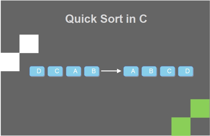
Quicksort in C follows the divide and conquer algorithm. In 1959, Tony Hoare, a British computer scientist, developed Quicksort, also known as partition-exchange sort. Since its publication in 1961, Quicksort has become one of the top algorithms to sort. It can be done in-place, which requires small additional memory to sort.

The Quicksort is the fastest known sort algorithm because of its highly optimized partitioning of an array of data into smaller arrays. An extensive array partition into two arrays holds values smaller than the specified value, say pivot, based on which the partition is made. Another array contains values more than the pivot value. Median-of-three partitioning is the best way to choose a suitable pivot element. Once a pivot has select, its position finalizes in the sorted array. It can’t change.

Quicksort breaks down the problem of sorting the entire array into smaller problems by breaking the array down. This technique of dividing the major problem into smaller problems is known as the dividing and conquering approach. For large sets of data, this algorithm is quite efficient as its average, and worst-case complexity is O(n2), and n is the number of items.

The hardest part of Quicksort is the partitioning of elements. The algorithm looks at the first element of the array (called the “pivot”). The process of placing the pivot in its final position is called partitioning. You can choose any element as the pivot and partition of the array. It will put all of the less than the pivot elements in the lower portion of the array and the elements higher than the pivot in the array’s upper part. When that is complete, it can put the pivot between those two sections, and quick sort will be able to sort the two areas separately.

For example: In the array {53, 38, 64, 15, 18, 9, 7, 26}, we take 26 as pivot. So after the first pass, the list will be changed like this. {7 9 18 15 26 64 38 53}

Therefore after the first pass, the pivot is set, with all the elements smaller to their left and all the elements larger than their right. Now, 7 9 18 15 and 63 38 53 are two separate arrays, and the same recursive logic applies to them, and we will continue to do that until the whole array has sort.

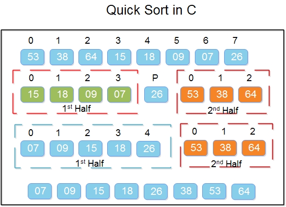
Below is a pictorial depiction of how quickly the given array is sorted.

In step 1, you choose the last element as pivot, which is 26, and you call for partitioning so that 26 place in its final position, and all the elements on the left are less than it, and on the right, all elements are greater than it.

Then we select the subarray to the left and the subarray to the right and choose the pivot. In the diagram above, we chose 07 as a pivot in the left and 64 as a pivot in the right array.

And we again call for partitioning.

This algorithm divides the list into three main parts:

1) Select an array element. This element refers to as a pivot.
2) Divide the unsorted element array into two arrays with values lower than the first subarray’s pivot. In the second subarray, all elements with values above the pivot (equal values can go anyway). This step is called the operation of the partition.

3) Recursively repeat step 2(until the sub-arrays are sorted) to the sub-array of smaller-value elements and higher-value elements. We implemented the same logic in the following C program.

C Program – Quicksort algorithm implementation
//Quicksort program in C
#includestdio.h> 
#include<stdbool.h> 
#define MAX 8 
int intArray[MAX] = {53, 38, 64, 15, 18, 9, 7, 26}; 
void printline(int count) { 
 int i; 
 for(i = 0;i <count-1;i++) { 
  printf("-"); 
 } 
  printf("-\n"); 
} 
void display() { 
 int i; 
 printf("["); 
 for(i = 0;i<MAX;i++) { 
  printf("%d ",intArray[i]); 
 } 
 printf("]\n"); 
} 
void swap(int n1, int n2) { 
 int temp = intArray[n1]; 
 intArray[n1] = intArray[n2]; 
 intArray[n2] = temp; 
} 
int partition(int left, int right, int pivot) { 
 int leftPointer = left -1; 
 int rightPointer = right; 
 while(true) { 
  while(intArray[++leftPointer] < pivot) { 
  //do nothing 
  } 
  while(rightPointer > 0 && intArray[--rightPointer] > pivot) { 
   //do nothing 
  } 
  if(leftPointer >= rightPointer) { 
    break; 
  } 
  else { 
   printf(" item swapped :%d,%d\n", intArray[leftPointer],intArray[rightPointer]); 
    swap(leftPointer,rightPointer); 
  } 
} 
 printf(" pivot swapped :%d,%d\n", intArray[leftPointer],intArray[right]); 
 swap(leftPointer,right); 
 printf("Updated Array: "); 
 display(); 
 return leftPointer; 
} 
 void quickSort(int left, int right) { 
  if(right-left <= 0) { 
    return; 
  } 
  else { 
   int pivot = intArray[right]; 
   int partitionPoint = partition(left, right, pivot); 
   quickSort(left,partitionPoint-1); 
   quickSort(partitionPoint+1,right); 
  } 
} 
main() { 
 printf("Input Array: "); 
 display(); 
 printline(50); 
 quickSort(0,MAX-1); 
 printf("Output Array: "); 
 display(); 
 printline(50); 
} 

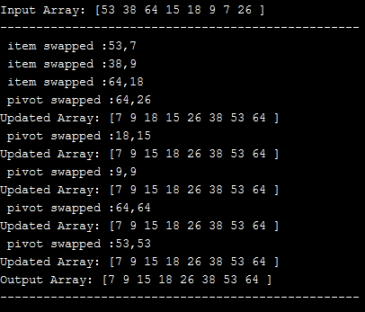
Output:

Complexity Analysis of Quick Sort

The time required to sort a total of n numbers in the quicksort algorithm shown in the following equation:

T(n) = T(k) + T(n-k-1) + (n) → (i)

The two recursive calls in the quicksort algorithm are T(k) and T(n-k-1). The last term n describes the partitioning process, while k represents the total number in the set, which is less than the pivot.

Note that the total time taken to complete a quicksort algorithm depends on the input array and the deployed partition strategy.

• Worst-Case: If the partition process always takes the smallest or largest element as the pivot, the worst case of a quick-sort algorithm is considered.

For example, in the above-mentioned quick sorting program in C, the worst case occurs if the last element is selected as the pivot point.
The equation (i) gets transformed for worst case of quick sort as follows:

T(n) = T(0) + T(n-1) + (n)
It can be written as:
T(n) = T(n-1) + (n)
Hence,T(n)worst case = O(n2)

• Average Case: Any quicksort cases that are not the worst-case or the best case is an average case.
To carry out the average quicksort case analysis, all possible permutations in the given array must be considered and the time taken for each permutation calculated. It’s a very difficult process.
A way around this problem is to consider the average case when the partitioning process puts (n/9) elements in one set and (9n/10) elements in the other one.

Therefore, equation (i) gets transformed into,T(n) = T(n/9) + T(9n/10) + (n) 
Solution to above mentioned recurrence relation will be,T(n) = (n log n)
Hence,T(n) average-case = O(n log n).

• Best Case:  The best case is when the partitioning process picks the middle element as the pivot.

Hence, equation (i) becomes,T(n) = 2T(n/2) + (n)
Using case 2 of Master Theorem,T(n) = (n log n)
Hence,T(n) best-case = O(n log n)

When to use and when to avoid Quick Sort ?

Use quick sort in the following scenarios:

When fast sorting is desired, quicksort has an average O(N log N) complexity, which is better than the bubble or insertion sort.

Avoid using quick sort when:

• If space is as limited as in embedded systems.
• Stable sorting is required when ordering elements from the final sorted list.