Excel has one exciting feature related to entering data into separate areas of working papers: you can select one or more areas in a worksheet and fill in this area or areas. Moreover, the filling is carried out only using the keyboard, while all manipulations are performed strictly within the selected area. It looks awe-inspiring when the area is disconnected; that is when the selected area consists of several ranges. [Read more…] about Working with a Selection in Excel 2010
Excel
Highlighting Areas in Excel 2010
Selecting an area in a worksheet is a trivial task. Usually, it does with the mouse. A left-click is carried out over one of the four corner cells of the area intended for selection, and when the button is held down, the entire area is captured (the area is highlighted in color except for the corner cell). In fig. illustrates the process of allocating a range of cells A1: E8. [Read more…] about Highlighting Areas in Excel 2010
Contextual Ribbon Tabs in Excel 2010
When working with various objects, contextual tabs can be added to the ribbon. They are available when the corresponding objects are selected and are intended for editing and managing them. In a given situation, the user, in addition to those listed above, can, for example, see tabs on the ribbon: Working with pictures (working with drawn objects), Working with diagrams (a tab for working with diagrams), Drawing tools (a tab for working with Images), Working with tables (working with tables), Working with SmartArt graphics (working with decorative text elements), Working with headers and footers (tab for working with headers and footers). As an illustration: after inserting an image into the working document and selecting it on the ribbon, another tab, Working with Pictures, appears. [Read more…] about Contextual Ribbon Tabs in Excel 2010
Customizing the Ribbon in Excel 2010
In Excel 2010, you can customize the ribbon. To do this, open the Excel Options window in the Customize the Ribbon section. [Read more…] about Customizing the Ribbon in Excel 2010
Active Label of a Ribbon Group in Excel 2010
In the lower right part of some groups, there is an active label, with the help of which many essential possibilities are realized. The specifics depend on the specific groups on the ribbon tabs. To activate the group label utility, you must click on it. [Read more…] about Active Label of a Ribbon Group in Excel 2010
Adding Ribbon Groups to the Quick Access Toolbar in Excel 2010
Even in the simplest version, the tape contains a sufficiently large number of tabs, which significantly slows down the work, primarily if icons are used in different places. We have already described how icons for individual commands are added to the Quick Access Toolbar. Excel 2010 can add icons for entire groups to the Quick Access Toolbar. [Read more…] about Adding Ribbon Groups to the Quick Access Toolbar in Excel 2010
Ribbon Tabs in Excel 2010
The ribbon is located in the upper part of the working window of the application and has the form shown in Figure.
The ribbon presented here contains eight standard tabs (Home, Insert, Page Layout, Formulas, Data, Review, View, and Developer), as well as one special tab, the File tab, used to make global system settings. Each standard tab consists of separate groups. Groups, in turn, contain controls. Some of them play the role of buttons, clicking on which leads to executing certain actions and commands. A large number of icons are essentially analogous to the menu. Clicking on such an icon leads to the expansion of the list of commands or submenu. In groups and tabs, the commands are selected mainly thematically, although there are some exceptions. [Read more…] about Ribbon Tabs in Excel 2010
Color Scheme in Excel 2010
An interesting enough innovation in the latest version of Excel 2010 is choosing colour schemes for displaying working documents. Here and throughout the book, a standard colour scheme with predominantly blue colours used. You can change it to a silver and dark colour scheme. The choice of a colour scheme performed in the Color scheme section of the Excel Settings window, where you need to select the desired item from the drop-down list. [Read more…] about Color Scheme in Excel 2010
Using the Preferences Window in Excel 2010
The view settings can be performed using the utilities of the settings window of the Excel Options application. To do this, click on the File tab and select the Options command. As a result, the settings window of the Excel Options application opens, which has several sections. The section is selected from the list on the left side of the window. In the figure below, the Excel Options window is open in the General area. [Read more…] about Using the Preferences Window in Excel 2010
Displaying the Grid and Indexing Fields
The table grid appears to be an interface element quite natural since it forms the user’s view of the Excel working document as a table. However, there is a mode in which such a grid not displayed. Usually, they switch to this mode if Excel is used as a text editor, although there can be many reasons. It is pretty easy to switch to the hidden mode of the table grid. It would help if you unchecked the option Group Grid Show tabs Application Ribbon View. [Read more…] about Displaying the Grid and Indexing Fields
Full Screen Mode in Excel 2010
There is a so-called full-screen document viewing mode, upon switching to which the working area of the document expands to the size of the active area of the computer screen. Switching to full-screen mode is carried out by clicking on the icon with the full-screen image in the Book view modes group of the View tab. [Read more…] about Full Screen Mode in Excel 2010
Status Bar in Excel 2010
The status bar is located at the bottom of the working window of Excel 2010, and at first glance, it may seem that it is mainly a decorative element. However, in Excel, the status bar is an efficient and highly functional interface element, skillful use of which significantly improves productivity and facilitates data processing. In Figure below shows what a standard Excel status bar might look like below.
![]()
The icons and controls on the right side of the status bar have already been described earlier (except, perhaps, the icon for switching to the pagination line display mode, but this will be done later). On the left side of the status bar, there is an indicator in which, if the document is ready for work (entering and editing data by the user), the message “Ready” is displayed. It is followed by an icon for switching to the macro recording mode. This element is described in the VBA Programming Part V. By and large, if an empty cell is selected in a working document, this will exhaust the elements, indicators, and icons displayed by default in the status bar. However, you can expand the functionality of the status bar using special settings.
To customize the status bar, right-click on it, as a result of which the Customize status bar list opens.
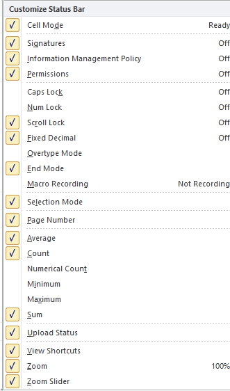
The list contains many items. By checking or unchecking the checkboxes, you can add or remove indicators and icons in the status bar. For some list items corresponding to the mode indicators, the current state (value) is displayed on the right side. In particular, for a message to appear in the status bar when you switch to the mode of entering uppercase letters, check the box next to the Caps Lock position. In this case, the status bar will look as shown in the figure below.
![]()
The aforementioned macro recording icon is displayed in the status line if the Macro recording checkbox is checked. As noted above, the group of view switching icons corresponds to the View mode shortcuts position, and the Scale and Scale slider positions are designed to display the thumbnail and a bar (with a slider) for selecting a scale.
The third section from the bottom in the Status bar settings list is quite interesting. In particular, if you check the boxes next to Average (calculating the Average), Count (number of non-empty cells), Minimum (minimum value), and Sum (Sum of cell values) and then in the working document.
Four additional messages will appear in the status bar if you want to select a range of non-empty cells.
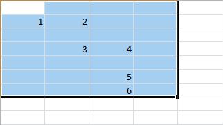
For the selected range of cells, the average value, the number of nonblank cells, the minimum value and the sum of the values in the cells are automatically calculated
More specifically: the Number of nonblank cells is determined in the selected range of cells, and the average value and the total sum of values in nonblank cells are calculated from these cells.
The Number of calculated parameters can be increased by checking the boxes next to the Number of numbers (the Number of non-empty cells with numeric values) and Maximum (maximum of values) positions in the status bar settings list. The result of applying such settings is illustrated in the figure below.
One of the cells contains a text value, so the total Number of nonblank cells is one less than the Number of nonblank cells with numeric values. When calculating the average and sum of values in cells, cells with text values are ignored.
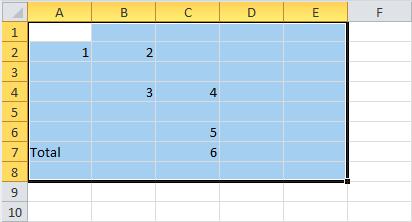
For the selected range of cells, the average value is automatically calculated,
number of nonblank cells, number of nonblank cells with numeric values, minimum number, maximum number, and sum of values in cells.
Formula Bar in Excel 2010
Formula bar in Excel 2010 is a large white field, marked on the left with an icon with a function image. [Read more…] about Formula Bar in Excel 2010
Name field in Excel 2010
An Excel worksheet contains a massive number of cells. If there is little data in the document and all of them are compactly placed in the upper left corner of the document, problems with determining the address of the currently active cell, as a rule, do not arise. However, it is often helpful, and sometimes just necessary, to quickly determine which cell is active. Helpful hints can be found in the name field in the formula bar, which is by default just below the ribbon on the left. [Read more…] about Name field in Excel 2010
Quick Access Toolbar
There is an access panel at the top of the working document – an echo of the toolbars used in previous versions of Excel. [Read more…] about Quick Access Toolbar
Spring Boot Interview Question
We’ll be covering the following topics in this tutorial:
Q. What exactly is the Spring Framework?
Spring is a general-purpose development framework for Java programs but is better suited for web and application development. It allows them to use much of the Java functionality out of other libraries while adding some new features. While it is an open-source application, it can be developed in an open manner using the Creative Common platform of the Spring Framework’s integral features. The majority of the functionality can be found in a Java Enterprise program. It has several plugins and APIs that augment the Java EE platform. [Read more…] about Spring Boot Interview Question
Working with Formula in Excel 2010
The worksheet would be nothing more than a plain tabular representation of data if there are no formulas. A formula is a set of instructions that must be typed into a cell. It performs some calculations and then displays the result in the cell. [Read more…] about Working with Formula in Excel 2010
Formatting Worksheets in Excel 2010
MS Excel offers a variety of printing sheet options, such as not printing cell gridlines. Choose Page Layout » Sheet Options Group » Gridlines » Check Print if you want your printout to include gridlines.
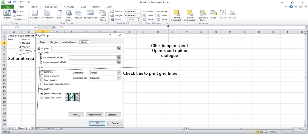 Options in Sheet Options Dialogue
- Print Area: This option allows you to specify the print area.
- Print Titles: You can place titles at the top of rows and the left of columns.
Print:
- Gridlines: When printing the worksheet, gridlines will appear.
- Black & White: Check this box to get the chart printed in black and white on your color printer.
- Draft quality: Select this check box to print the chart in draft quality on your printer.
- Print Rows & Column Heading: Check this box to print rows and column headings.
Page Order:
- Down, then Over: The down pages are printed first, followed by the right pages.
- Over, then Down: It prints the right pages first, then the down pages.
We’ll be covering the following topics in this tutorial:
Adjust Margins
The margins of the printed page and the extent of unprinted areas. In MS Excel, all printed pages have the same margins. Different margins cannot be defined for different pages.
Margins can be set in a variety of ways, as detailed below.
- Select Normal, Broad, Narrow, or Custom Setting from the Page Layout » Page Setup » Margins drop-down list.
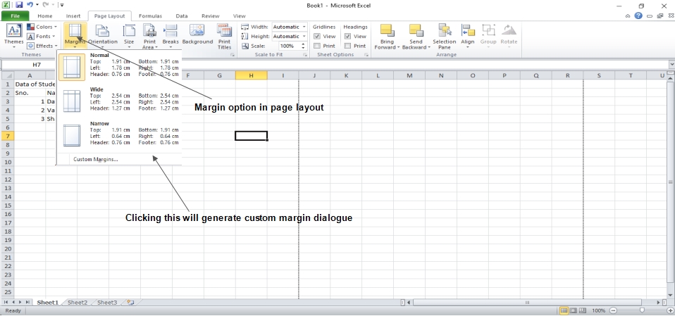
- These options are available when creating a report or selecting printing.
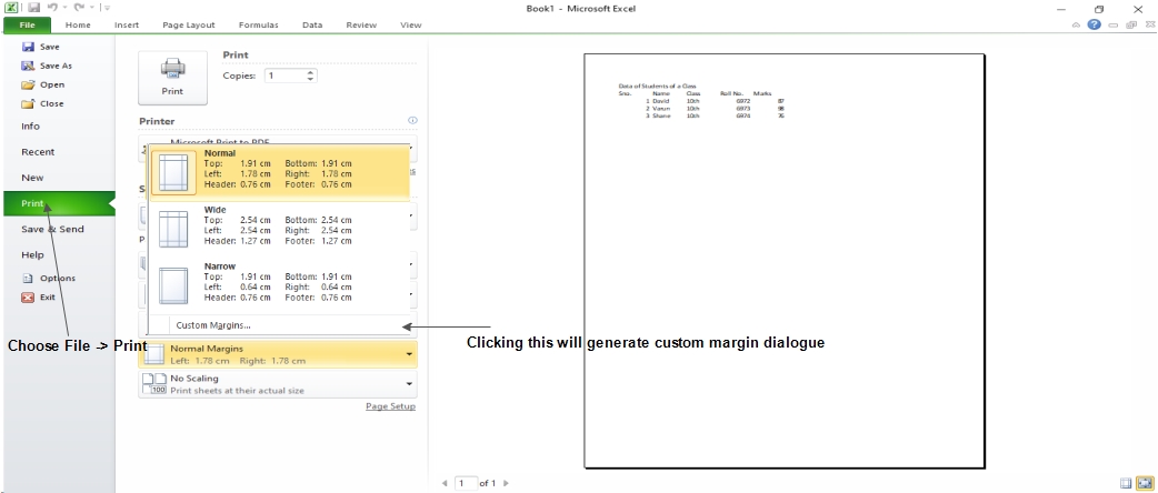 If none of the provided settings are satisfactory, please select Custom Margins from the Page Setup dialog box to display the Margins tab.
Center on Page
By default, Excel aligns the printed page at the top and left margins. If you want the output to be centered vertically or horizontally, select the appropriate check box in the Center on Page section of the Margins tab as shown in the above screenshot.
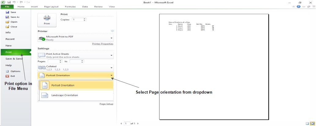
Page Orientation
The orientation of output on a page is referred to as page orientation. The onscreen page breaks adjust automatically to match the new paper orientation when you change the orientation.
Types of Page Orientation
- Portrait: To print tall pages, use portrait mode (the default).
- Landscape: Use this setting to print large pages.
When you have a large selection that won’t fit on a vertically oriented website, landscape orientation comes in handy.
Changing Page Orientation
- Choose Page Layout » Page Setup » Orientation » Portrait or Landscape.
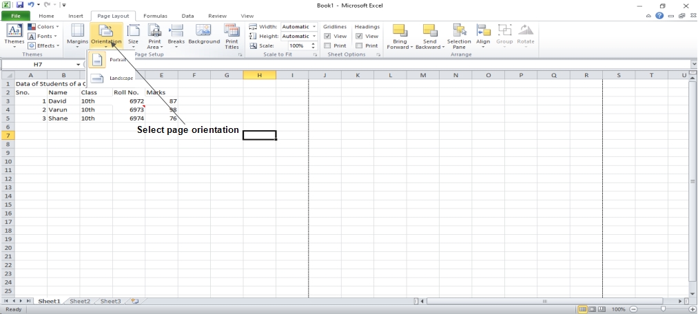
- Choose File » Print.
Header & Footer
The information that appears at the top of each printed page is referred to as a header, and the information that appears at the bottom of each printed page is referred to as footer.
New workbooks are produced without headers or footers by default.
Adding Header and Footer
- Choose Page Setup Dialog Box » Header or Footer Tab.
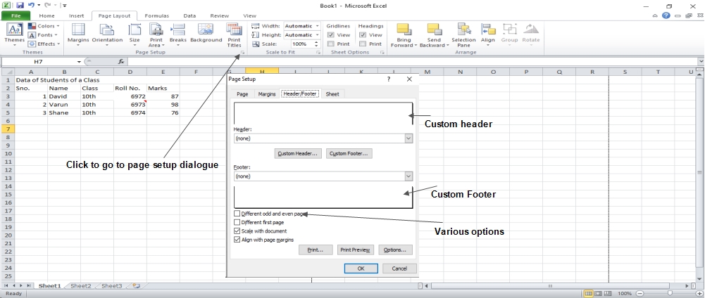
You can choose the predefined header and footer or create your custom ones.
- &[Page] : Displays the page number.
- &[Pages] : Displays the total number of pages to be printed.
- &[Date] : Displays the current date.
- &[Time] : Displays the current time.
- &[Path]&[File] : Displays the workbook’s complete path and filename.
- &[File] : Displays the workbook name.
- &[Tab] : Displays the sheet’s name.
Other Header and Footer Options
The Header & Footer » Design » Options group contains controls that let you specify other options when a header or footer is selected in Page Layout view:
- Different First Page: Choose this option to have the first printed page have a different header or footer.
- Different Odd and Even Pages: Select this option to define a different header or footer for odd and even pages.
- Scale with Document: When this option is selected, the font size in the header and footer will be adjusted. If the paper is scaled when typed, this would be the case. By default, this option is turned on.
- Align with Page Margins: If this option is selected, the left header and footer will be aligned with the left margin, and the right header and footer with the right margin. By default, this option is turned on.
Insert Page Break
If you don’t want a row to print on a page by itself or you don’t want a table header row to be the last line on a page. MS Excel gives you precise control over page breaks.
MS Excel handles page breaks automatically, but sometimes you may want to force a page break either a vertical or a horizontal one, so that the report prints the way you want.
For example, if your worksheet consists of several distinct sections, you may want to print each section on a separate sheet of paper.
Inserting Page Breaks
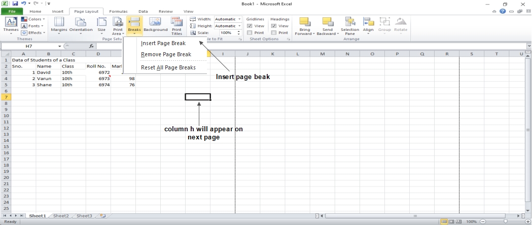
Insert Horizontal Page Break: Select cell A14 to insert a horizontal page break, for example, if you want row 14 to be the first row of a new page. Choose Page Layout » Page Setup Group » Breaks » Insert Page Break.
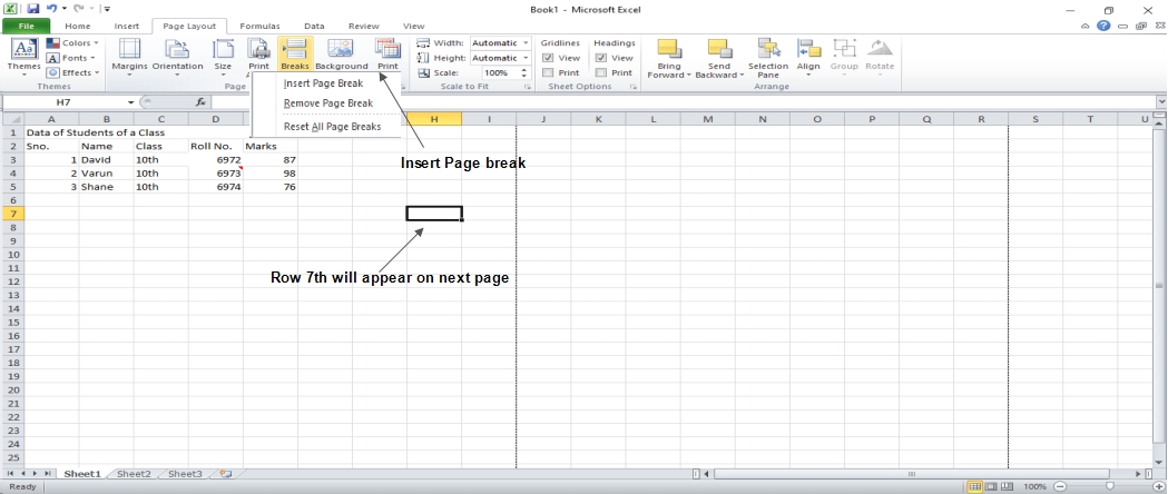
Insert a vertical page break: Make sure the pointer is in row 1 in this situation.
Choose from the following options: Page Layout » Page Setup » Breaks » Establish a page break by inserting a page break.
Removing Page Breaks
- If you’ve added a page break, remove it: Choose Page Layout » Page Setup » Breaks » and then transfer the cell pointer to the first row beneath the manual page break. Page Break should be removed.
- Remove all page breaks manually: Choose from the following options: Page Layout » Page Setup » Breaks » All page breaks should be reset.
Set Background
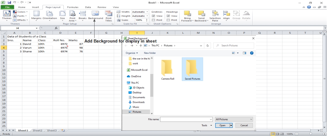
You can’t get a background image on your printouts, unfortunately. The Page Layout » Page Setup » Background command might have caught your attention. This button brings up a dialog box where you can choose a picture to use as a backdrop. This control’s placement among the other print-related commands is extremely misleading. On a worksheet, background images are never printed.
Alternative to Placing Background
- You can change the transparency of a Shape, WordArt, or a picture on your worksheet. The picture should then be copied to all printed sheets.
• An object may be placed in the page header or footer.
Freezing Panes
When you set up a worksheet with row or column headings, you won’t be able to see them if you scroll down or to the right. The freezing panes feature in MS Excel is a useful solution to this problem. When scrolling through the worksheet, freezing panes leaves the headings visible.
Using Freeze Panes
Follow the steps mentioned below to freeze panes.
- Freeze the first row, the first column, or the row below it, or the column right to the place you want to freeze.
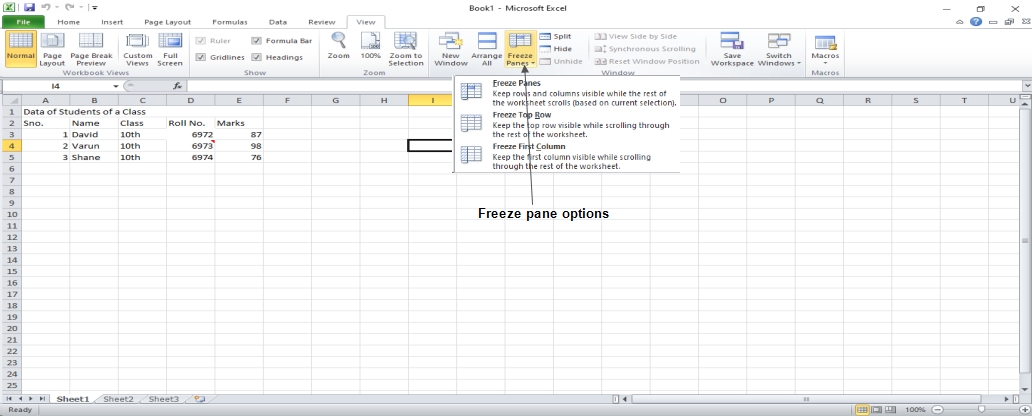
- Choose View Tab » Freeze Panes.
- Select the suitable option:
- Freeze Panes: To freeze area of cells.
- Freeze Top Row: To freeze first row of worksheet.
- Freeze First Column: To freeze first Column of worksheet.
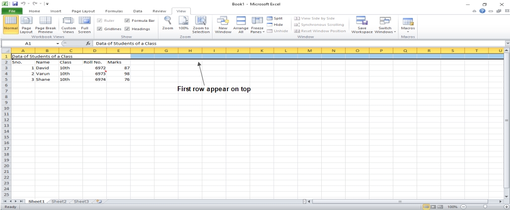
- If you select Freeze top row, the first row will appear at the top, even after scrolling. Take a look at the image below.
 Unfreeze Panes
To unfreeze Panes, choose View Tab » Unfreeze Panes.
Conditional Formatting
The Conditional Formatting function in Microsoft Excel 2010 allows you to format a set of values such that values outside of those bounds are automatically formatted.
Choose Home Tab » Style Group » Conditional Formatting Dropdown.
Various Conditional Formatting Options
- Highlight Cells Rules: Opens a continuation menu with a variety of options to define the formatting rules that highlight cells in the selection of cells that include certain values, text or dates, or that that have values greater than or less than a particular value, or that fall within a certain range of values.
Suppose you want to find cells with a value of 0 and color them red. Choose Range of Cell » Home Tab » Conditional Formatting DropDown » Highlight Cell Rules » Equal To.
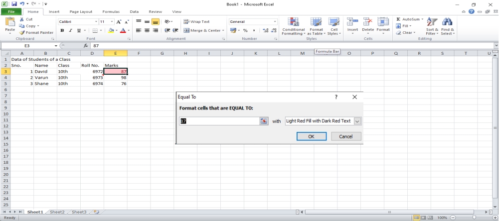
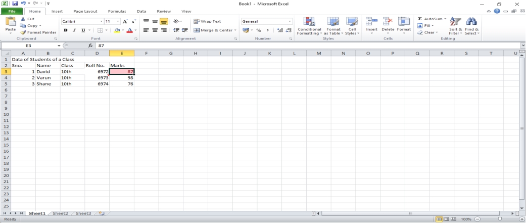
After Clicking OK, the cells with value zero are marked as red.
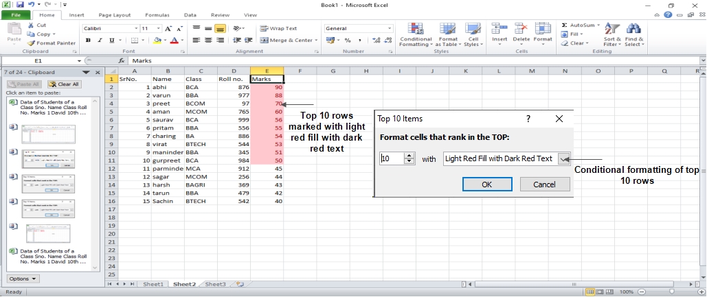
Top/Bottom Rules: Opens a continuation menu with a variety of options to define the formatting rules that highlight upper and lower values, percentages, and above and below average values in the range of cells.
Suppose you want to highlight the top 10% rows, you can do this with the Top/Bottom rules.
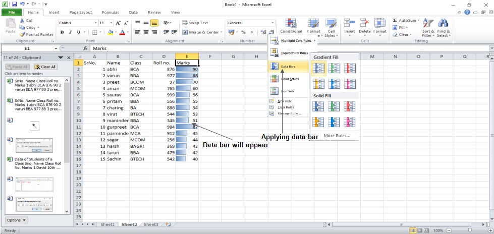
Data Bars: Opens a palette of different color data bars that you can add to the set of cells to show their values relative to each other by clicking on the data bar thumbnail.
With this conditional formatting, the data bars will be displayed in each cell.
Color Scales: It opens a palette of different three-and two-tone scales that can be applied to the set of cells to show their values relative to each other by clicking on the color scale thumbnail.
See the below screenshot with Color Scales, conditional formatting applied.
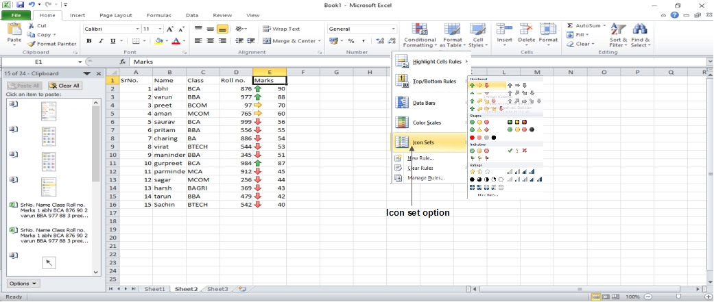
Icon Sets: It displays a palette of various icon sets that you can add to the cell selection to show their relative values by clicking the icon set.
See the below screenshot with Icon Sets, conditional formatting applied.
- New Rule: This option opens the New Formatting Rule dialog box, where you can create a custom conditional formatting rule for the cell range.
- Clear Rules: It opens a new menu where you can delete conditional formatting rules for the selected cells, the entire worksheet, or only the current data table by selecting the Selected Cells option, the Entire Sheet option, or the This Table option.
- Manage Rules: This option opens the Conditional Formatting Rules Manager dialog box, where you can edit and delete specific rules as well as change their rule precedence by moving them up or down in the Rules list box.
Formatting Cells in Excel 2010
MS Excel Cell can carry various types of data such as Numbers, Currency, Dates, etc. You can set the cell type in various ways including the following methods: [Read more…] about Formatting Cells in Excel 2010
Undo & Redo Changes in Excel 2010
Using the Undo command in Excel 2010, you can undo almost every action. We can reverse the changes in two ways. [Read more…] about Undo & Redo Changes in Excel 2010
Add Text Box in Excel 2010
Text boxes are special graphic objects which combine text with a rectangular graphic object. The text in rectangular boxes and cell comments are identical in showing text. But when cell comments are selected, the comments are shown via the cell. [Read more…] about Add Text Box in Excel 2010
Insert Comments in Excel 2010
In Excel 2010, adding a comment to a cell makes it easier to understand what the cell’s purpose is, what input it should accept, and so on. It helps in accurate documentation. Select a cell and perform any of the actions listed below to add a comment to it. [Read more…] about Insert Comments in Excel 2010
Special Symbols in Excel 2010
You must use the Symbols option if you want to insert symbols or special characters that are not available on the keyboard. [Read more…] about Special Symbols in Excel 2010
Paginated View in Excel 2010
The same documents may look completely different on a computer screen and when printed. This problem is especially relevant when working with Excel because, as already noted, the workspace is not paginated by default. Therefore, when entering data into cells of a worksheet, it is not always easy to predict how the data will be presented and grouped in printed form. Nevertheless, this problem is easily fixed, and there are several ways to fix it. Here we will describe the most simple and effective one. It is about switching to the pagination mode of the work area. It is enough to click on a special icon on the status bar – the central one of the three icons to the left of the scale selection switch. [Read more…] about Paginated View in Excel 2010
Zoom IN/OUT in Excel 2010
The data in the table is perceived differently depending on the display scale of the stage (that is, the area of cells). The ribbon version of Excel provides a very convenient way to set the desired scale: there is a special bar with a slider for selecting the display scale in the status bar. A functional text field (scale indicator) is placed next to the strip, displaying the display scale set by the user (by default, the value is 100%). The scale setting bar is shown in Fig below.
Spell Checker in Excel 2010
Excel 2010 has a spell checker that will allow us to detect spelling errors within our spreadsheet. Excel searches every word in its dictionary, and any word that it does not find will consider it a possible wrong word. [Read more…] about Spell Checker in Excel 2010
Find & Replace in Excel 2010
When we handle a significant amount of data, sometimes we need to locate specific data in the book. To facilitate this task, there is a search tool. We will find it in the tab Home > Search and select. [Read more…] about Find & Replace in Excel 2010
Copy & Paste in Excel 2010
MS Excel offers the ability to copy paste in various ways. The best way to copy the paste is as follows. [Read more…] about Copy & Paste in Excel 2010
Rows & Columns in Excel 2010
The tabular format of MS Excel is made up of rows and columns.
- Column runs vertically, while Row runs horizontally.
- The row number, which runs vertically down the left side of the sheet, identifies each row.
- The column header, which runs horizontally across the top of the sheet, identifies each column.
