Formatting Worksheets in Excel 2010

MS Excel offers a variety of printing sheet options, such as not printing cell gridlines. Choose Page Layout » Sheet Options Group » Gridlines » Check Print if you want your printout to include gridlines.

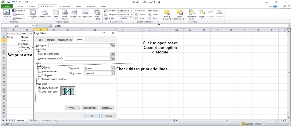Options in Sheet Options Dialogue

• Print Area: This option allows you to specify the print area.
• Print Titles: You can place titles at the top of rows and the left of columns.

Print:

• Gridlines: When printing the worksheet, gridlines will appear.
• Black & White: Check this box to get the chart printed in black and white on your color printer.
• Draft quality: Select this check box to print the chart in draft quality on your printer.
• Print Rows & Column Heading: Check this box to print rows and column headings.

Page Order:

• Down, then Over: The down pages are printed first, followed by the right pages.
• Over, then Down: It prints the right pages first, then the down pages.

Adjust Margins

The margins of the printed page and the extent of unprinted areas. In MS Excel, all printed pages have the same margins. Different margins cannot be defined for different pages.

Margins can be set in a variety of ways, as detailed below.

• Select Normal, Broad, Narrow, or Custom Setting from the Page Layout » Page Setup » Margins drop-down list.

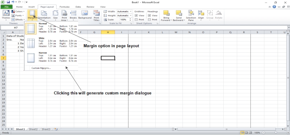
• These options are available when creating a report or selecting printing.

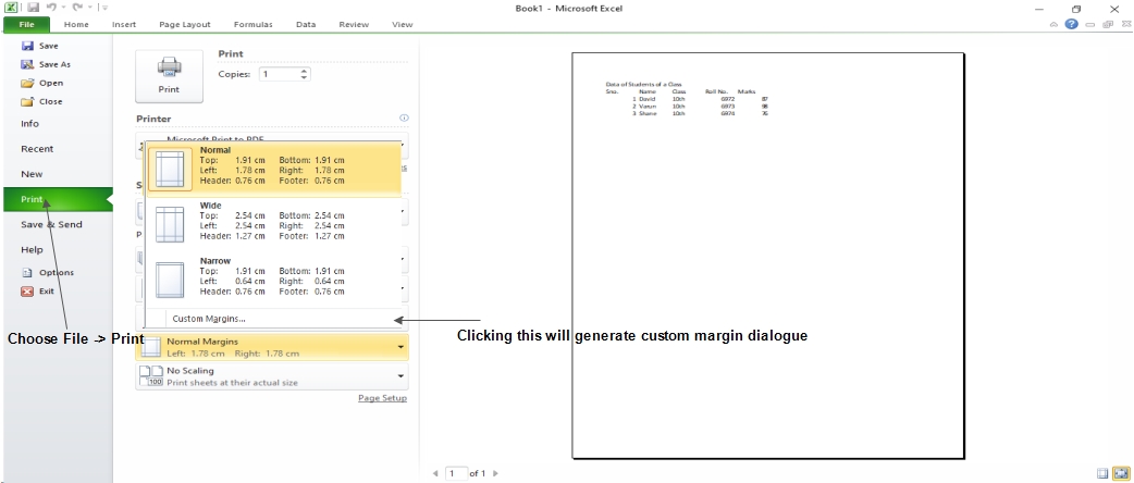If none of the provided settings are satisfactory, please select Custom Margins from the Page Setup dialog box to display the Margins tab.

Center on Page   

By default, Excel aligns the printed page at the top and left margins. If you want the output to be centered vertically or horizontally, select the appropriate check box in the Center on Page section of the Margins tab as shown in the above screenshot.

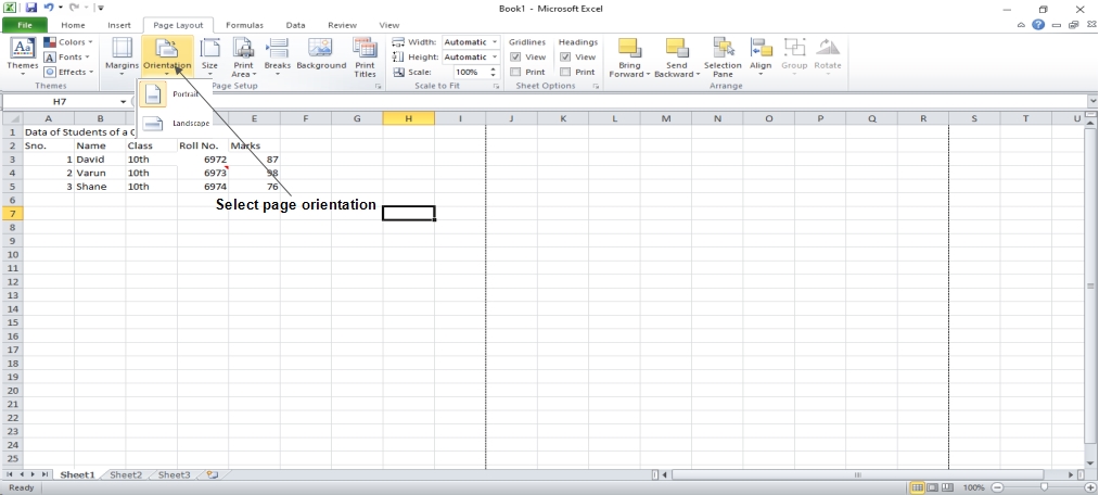
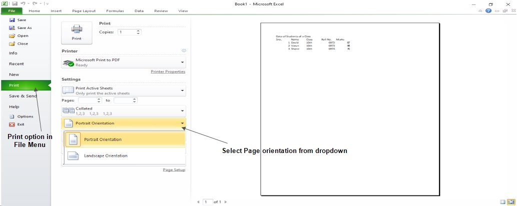
Page Orientation 

The orientation of output on a page is referred to as page orientation. The onscreen page breaks adjust automatically to match the new paper orientation when you change the orientation.

Types of Page Orientation          

• Portrait: To print tall pages, use portrait mode (the default).
• Landscape: Use this setting to print large pages.

When you have a large selection that won’t fit on a vertically oriented website, landscape orientation comes in handy.

Changing Page Orientation

• Choose Page Layout » Page Setup » Orientation » Portrait or Landscape.

• Choose File » Print.

Header & Footer

The information that appears at the top of each printed page is referred to as a header, and the information that appears at the bottom of each printed page is referred to as footer.

New workbooks are produced without headers or footers by default.

Adding Header and Footer

• Choose Page Setup Dialog Box » Header or Footer Tab.

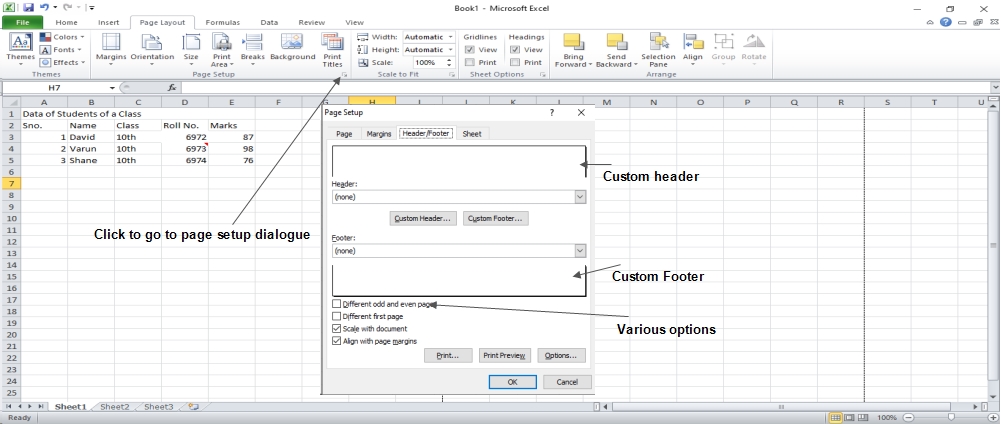
You can choose the predefined header and footer or create your custom ones.

• &[Page] : Displays the page number.
• &[Pages] : Displays the total number of pages to be printed.
• &[Date] : Displays the current date.
• &[Time] : Displays the current time.
• &[Path]&[File] : Displays the workbook’s complete path and filename.
• &[File] : Displays the workbook name.
• &[Tab] : Displays the sheet’s name.

Other Header and Footer Options

The Header & Footer » Design » Options group contains controls that let you specify other options when a header or footer is selected in Page Layout view:

• Different First Page: Choose this option to have the first printed page have a different header or footer.
• Different Odd and Even Pages: Select this option to define a different header or footer for odd and even pages.
• Scale with Document: When this option is selected, the font size in the header and footer will be adjusted. If the paper is scaled when typed, this would be the case. By default, this option is turned on.
• Align with Page Margins: If this option is selected, the left header and footer will be aligned with the left margin, and the right header and footer with the right margin. By default, this option is turned on.

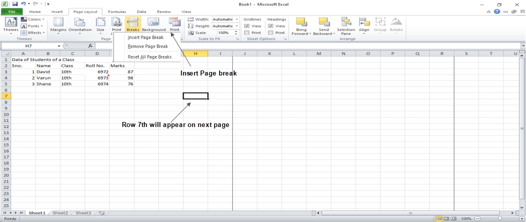
Insert Page Break  

If you don’t want a row to print on a page by itself or you don’t want a table header row to be the last line on a page. MS Excel gives you precise control over page breaks.

MS Excel handles page breaks automatically, but sometimes you may want to force a page break either a vertical or a horizontal one, so that the report prints the way you want.

For example, if your worksheet consists of several distinct sections, you may want to print each section on a separate sheet of paper.

Inserting Page Breaks

Insert Horizontal Page Break: Select cell A14 to insert a horizontal page break, for example, if you want row 14 to be the first row of a new page. Choose Page Layout » Page Setup Group » Breaks » Insert Page Break.

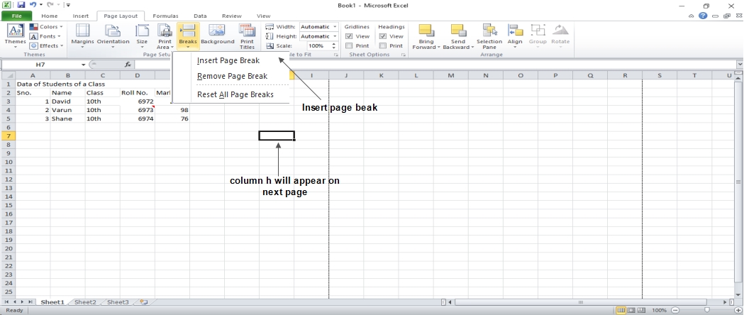
Insert a vertical page break: Make sure the pointer is in row 1 in this situation.

Choose from the following options: Page Layout » Page Setup » Breaks » Establish a page break by inserting a page break.

Removing Page Breaks     

• If you’ve added a page break, remove it: Choose Page Layout » Page Setup » Breaks » and then transfer the cell pointer to the first row beneath the manual page break. Page Break should be removed.
• Remove all page breaks manually: Choose from the following options: Page Layout » Page Setup » Breaks » All page breaks should be reset.

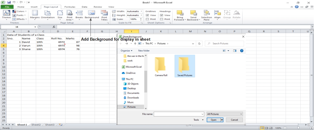
Set Background   

You can’t get a background image on your printouts, unfortunately. The Page Layout » Page Setup » Background command might have caught your attention. This button brings up a dialog box where you can choose a picture to use as a backdrop. This control’s placement among the other print-related commands is extremely misleading. On a worksheet, background images are never printed.

Alternative to Placing Background   

• You can change the transparency of a Shape, WordArt, or a picture on your worksheet. The picture should then be copied to all printed sheets.

• An object may be placed in the page header or footer.

Freezing Panes

When you set up a worksheet with row or column headings, you won’t be able to see them if you scroll down or to the right. The freezing panes feature in MS Excel is a useful solution to this problem. When scrolling through the worksheet, freezing panes leaves the headings visible.

Using Freeze Panes   

Follow the steps mentioned below to freeze panes.

• Freeze the first row, the first column, or the row below it, or the column right to the place you want to freeze.
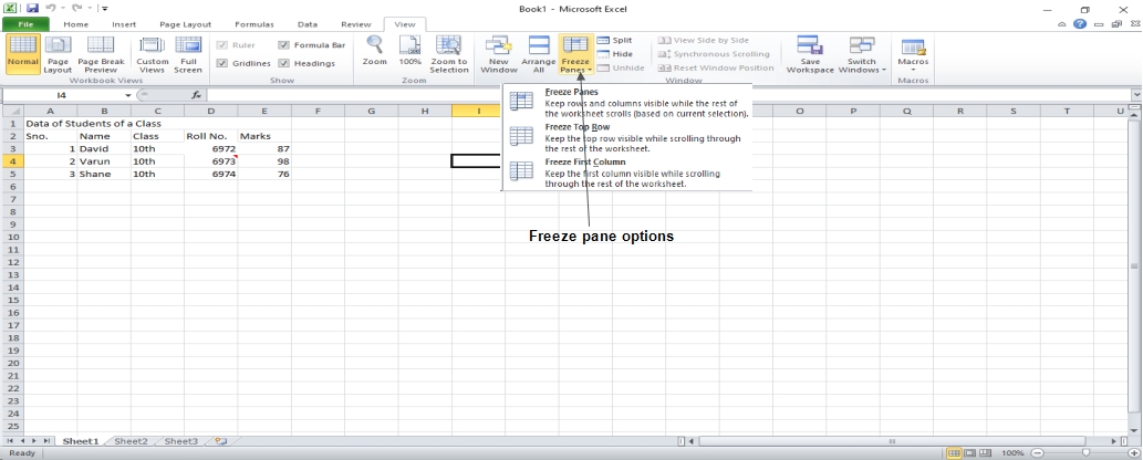
• Choose View Tab » Freeze Panes.
• Select the suitable option:
• Freeze Panes: To freeze area of cells.
• Freeze Top Row: To freeze first row of worksheet.
• Freeze First Column: To freeze first Column of worksheet.

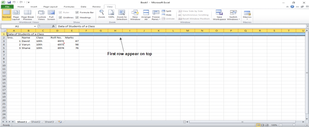
• If you select Freeze top row, the first row will appear at the top, even after scrolling. Take a look at the image below.

Unfreeze Panes  

To unfreeze Panes, choose View Tab » Unfreeze Panes.

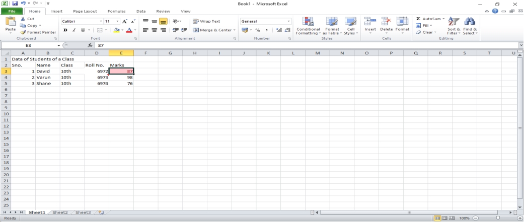
Conditional Formatting

The Conditional Formatting function in Microsoft Excel 2010 allows you to format a set of values such that values outside of those bounds are automatically formatted.

Choose Home Tab » Style Group » Conditional Formatting Dropdown.

Various Conditional Formatting Options

• Highlight Cells Rules: Opens a continuation menu with a variety of options to define the formatting rules that highlight cells in the selection of cells that include certain values, text or dates, or that that have values greater than or less than a particular value, or that fall within a certain range of values.

Suppose you want to find cells with a value of 0 and color them red. Choose Range of Cell » Home Tab » Conditional Formatting DropDown » Highlight Cell Rules » Equal To.

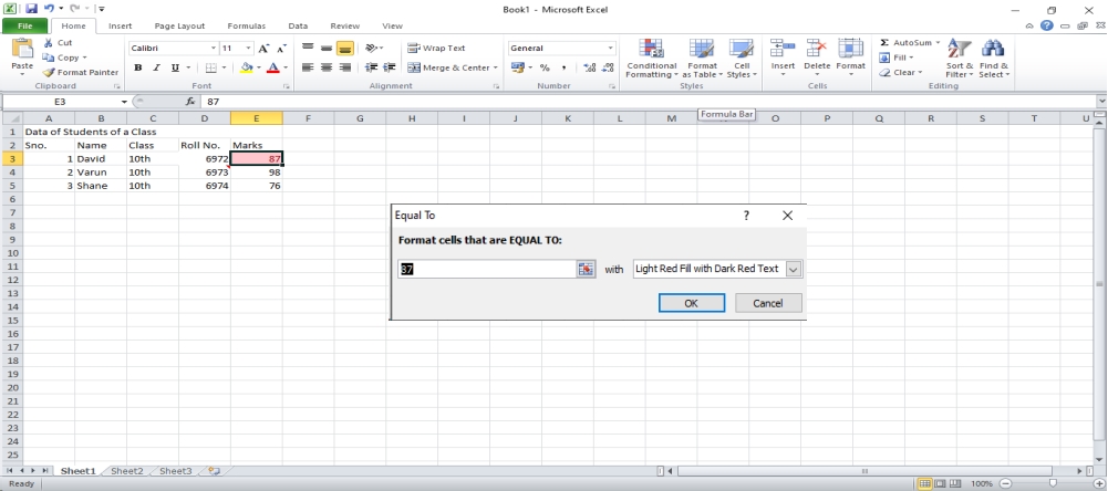
After Clicking OK, the cells with value zero are marked as red.

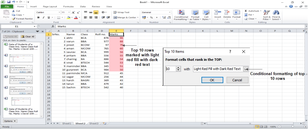
Top/Bottom Rules: Opens a continuation menu with a variety of options to define the formatting rules that highlight upper and lower values, percentages, and above and below average values in the range of cells.

Suppose you want to highlight the top 10% rows, you can do this with the Top/Bottom rules.

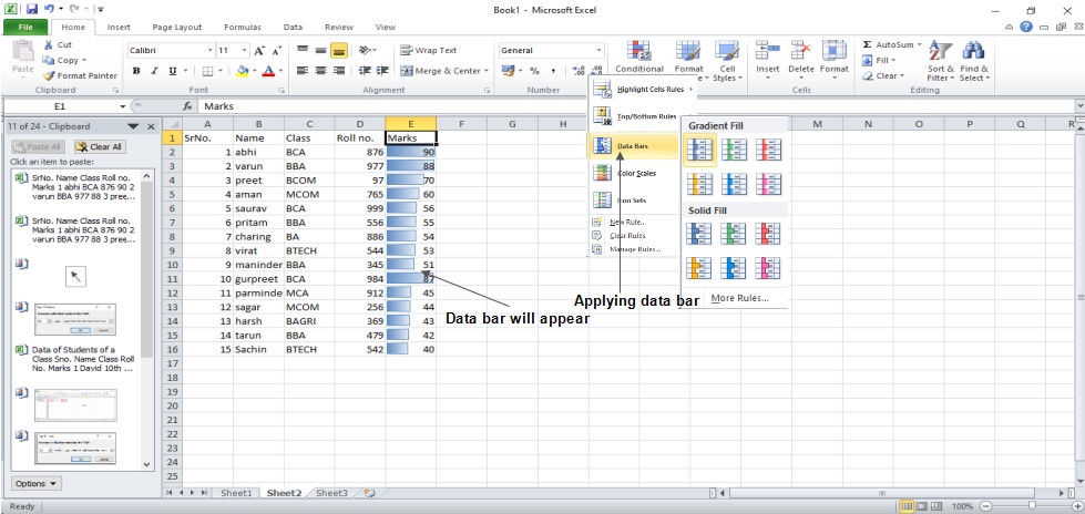
Data Bars: Opens a palette of different color data bars that you can add to the set of cells to show their values relative to each other by clicking on the data bar thumbnail.

With this conditional formatting, the data bars will be displayed in each cell.

Color Scales: It opens a palette of different three-and two-tone scales that can be applied to the set of cells to show their values relative to each other by clicking on the color scale thumbnail.

See the below screenshot with Color Scales, conditional formatting applied.

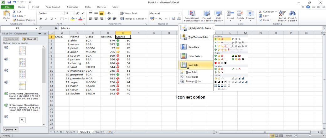
Icon Sets: It displays a palette of various icon sets that you can add to the cell selection to show their relative values by clicking the icon set.

See the below screenshot with Icon Sets, conditional formatting applied.

• New Rule: This option opens the New Formatting Rule dialog box, where you can create a custom conditional formatting rule for the cell range.
• Clear Rules: It opens a new menu where you can delete conditional formatting rules for the selected cells, the entire worksheet, or only the current data table by selecting the Selected Cells option, the Entire Sheet option, or the This Table option.
• Manage Rules: This option opens the Conditional Formatting Rules Manager dialog box, where you can edit and delete specific rules as well as change their rule precedence by moving them up or down in the Rules list box.